Prokudin-Gorskii Photo Collection

Sergei Mikhailovich Prokudin-Gorskii (1863–1944), a Russian photographer and chemist, is best known for his work in early color photography. While color photography was still in its infancy, Prokudin-Gorskii created a camera capable of taking color images by capturing separate black-and-white photographs through red, green, and blue filters. Prokudin-Gorskii believed that eventually, these images would be able to be viewed in color through a specialized projector.

Although Prokudin-Gorskii’s dream of color photography was never realized, his work has been digitized and colorized by various individuals and organizations. The Library of Congress has a collection of over 2,000 of his images, which can be viewed here.

In this project, my goal is to colorize his one-of-a-kind images.

Original Images

As we can see, Prokudin-Gorskii’s pictures were taken in three separate black-and-white images, each with a red, green, or blue filter. The top exposure has been shot with a blue filter, the middle with a green filter, and the bottom with a red filter.

From a first glance, it is clear that the channels are not perfectly aligned, nor are their dimensions always the same. In the Onion Church’s blue channel, part of the onion dome is cut off, and the red channel seems cut short on both the top and bottom. The train’s entire slide appears larger than the Onion Church’s.

Naive Approach

To colorize the images, I first tried a naive approach. I simply stacked the three images on each other and used the red, green, and blue channels to create a color image.

# Read in the image
img = skio.imread(img_name)

# Convert to double
img = sk.img_as_float(img)

# Compute the height of each channel (just 1/3 of total)
height = np.floor(img.shape[0] / 3.0).astype(np.int32)

# Separate color channels
b = img[:height]
g = img[height: 2*height]
r = img[2*height: 3*height]

#Naive Alignment
stacked = np.dstack((r,g,b))

The results of this naive approach can be seen below.

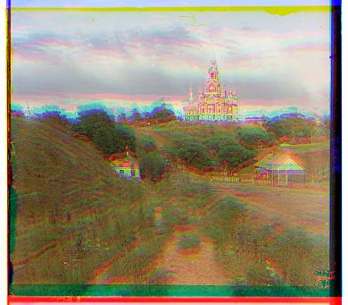
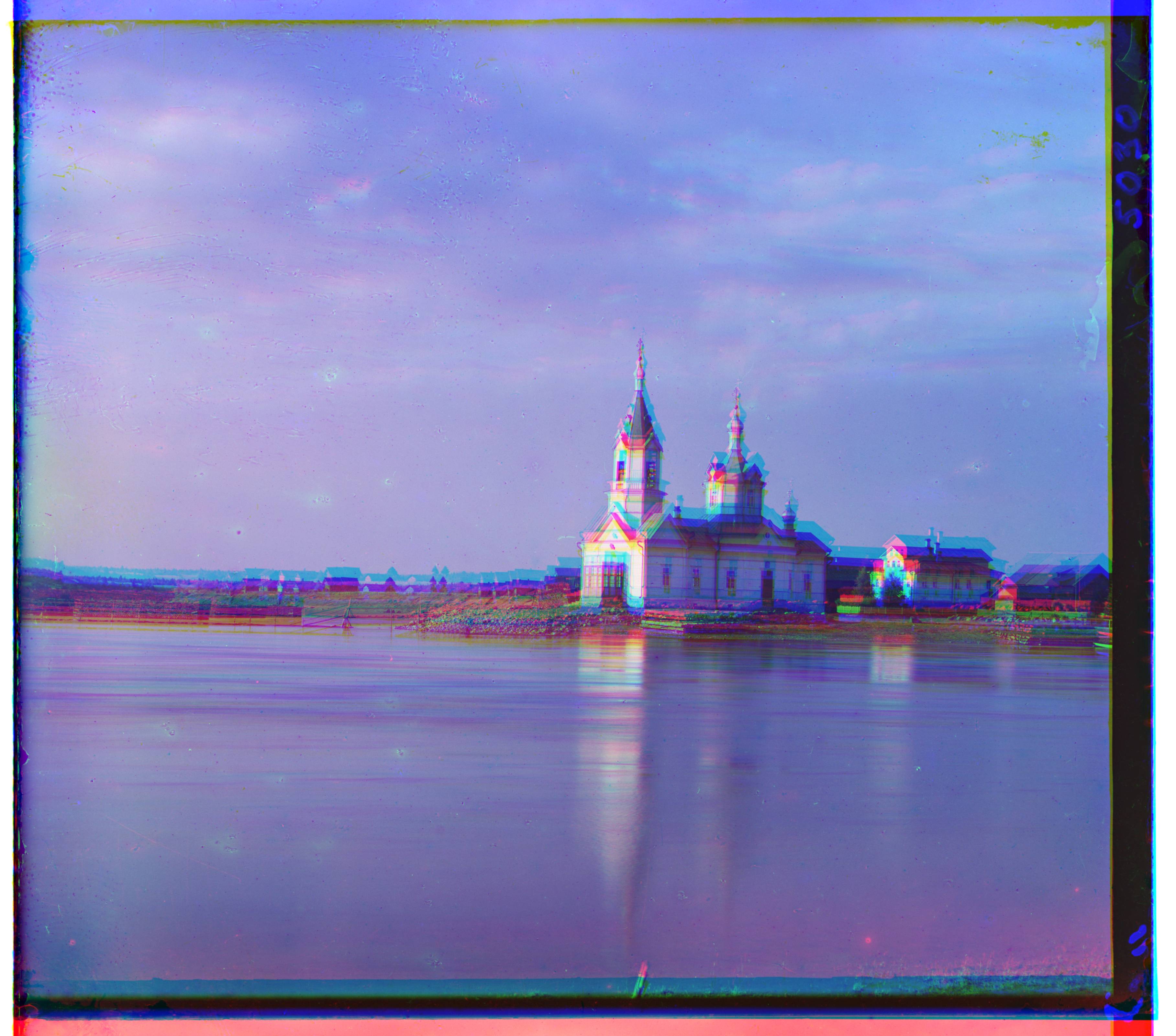
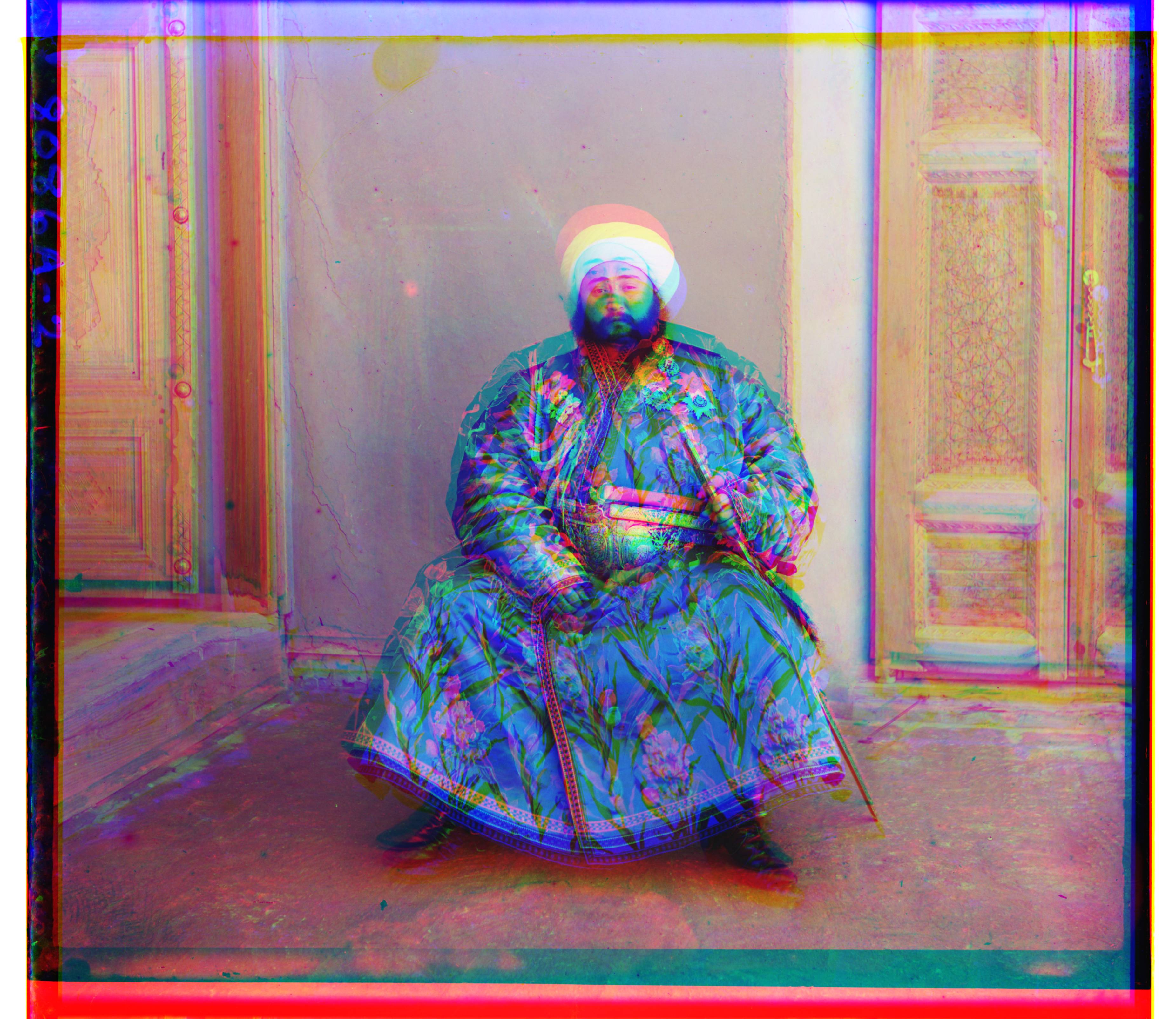
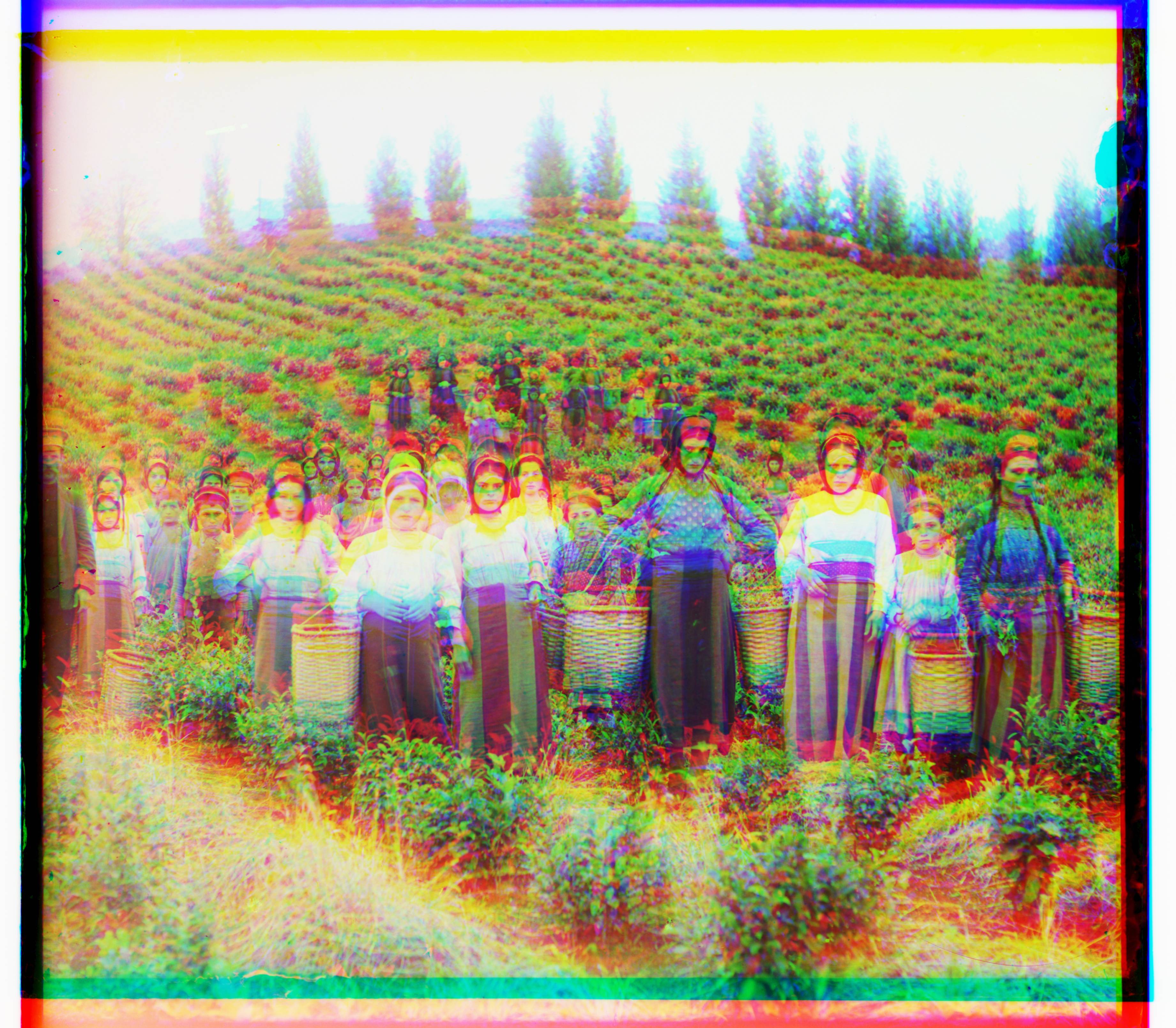
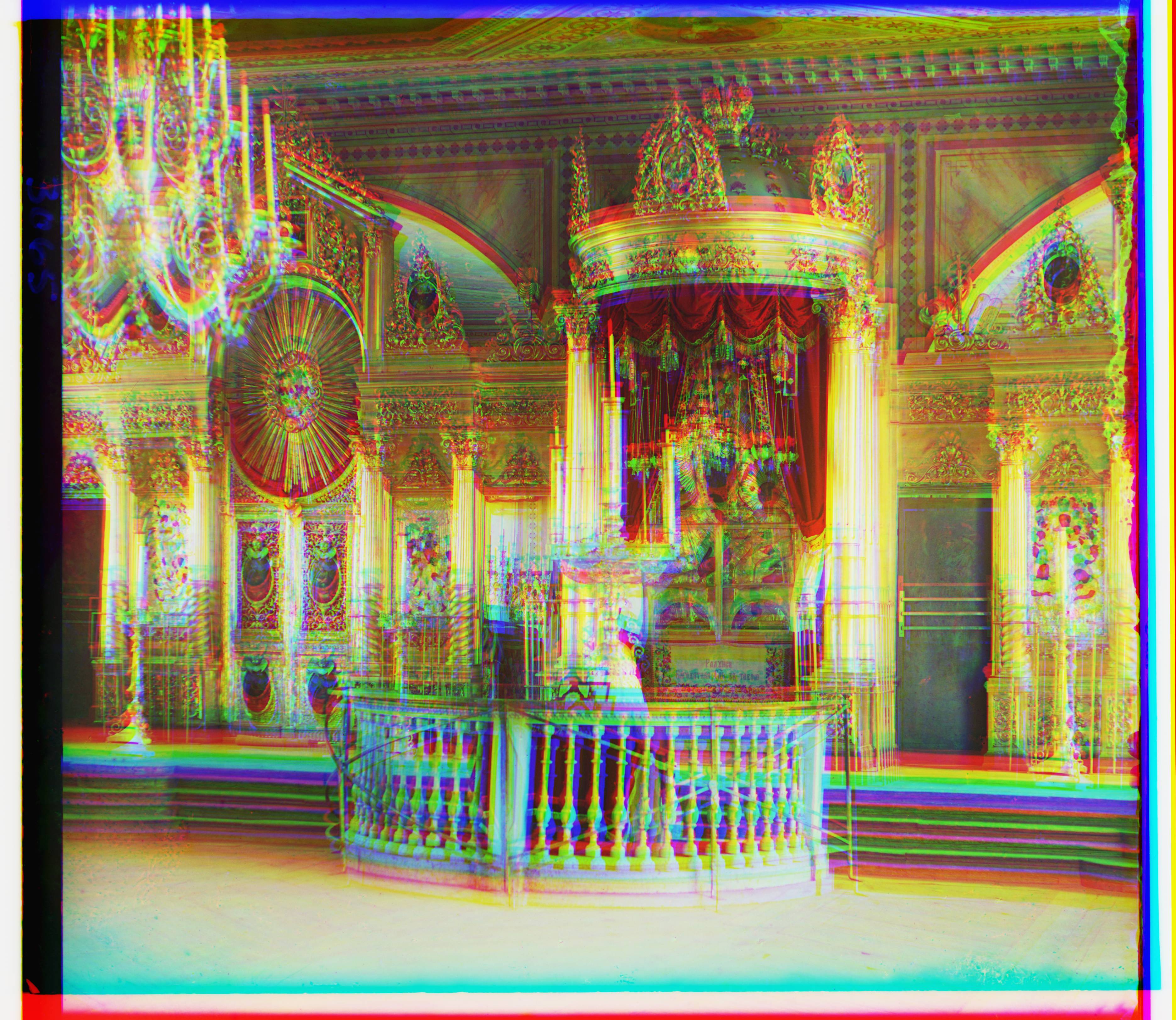
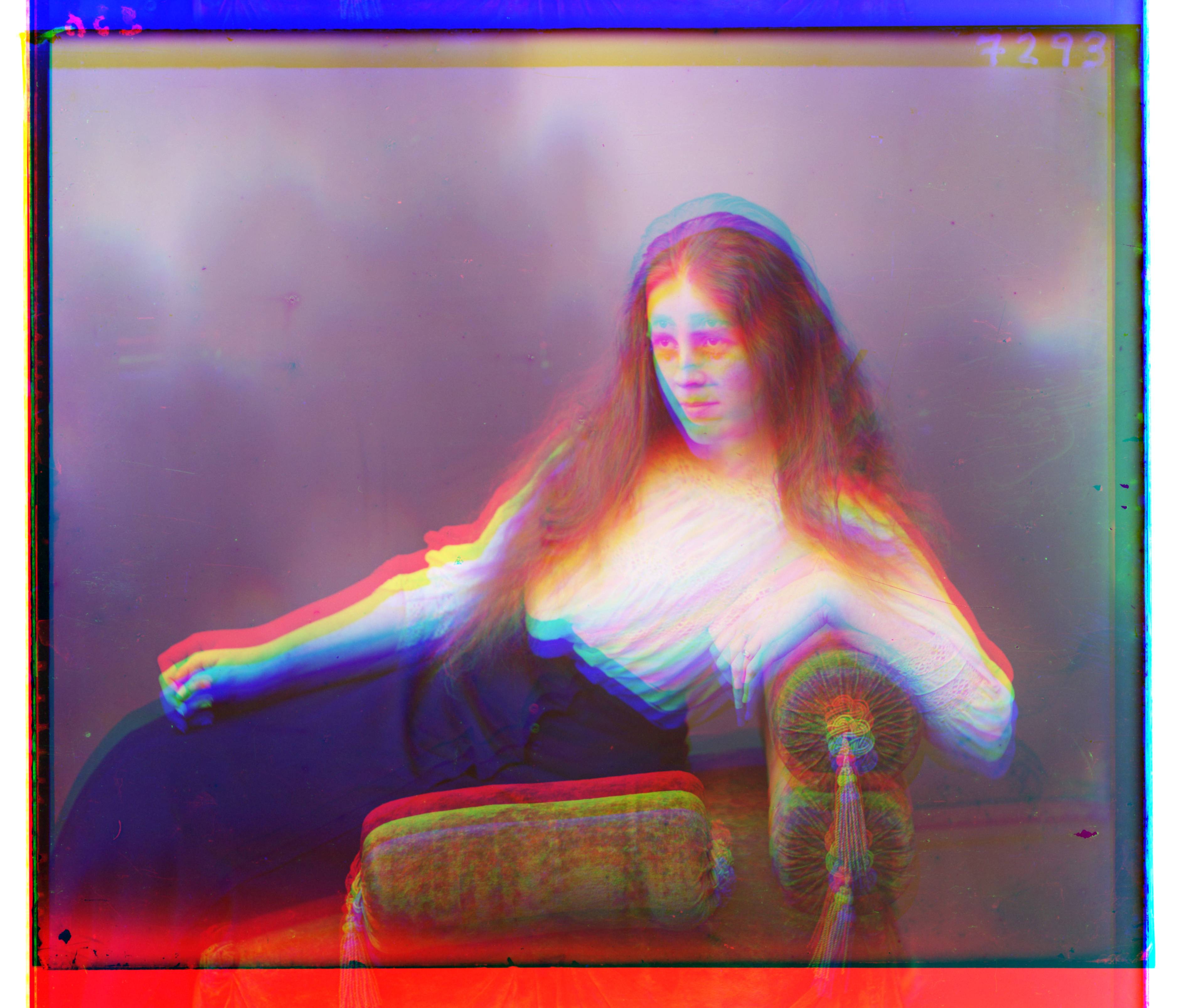
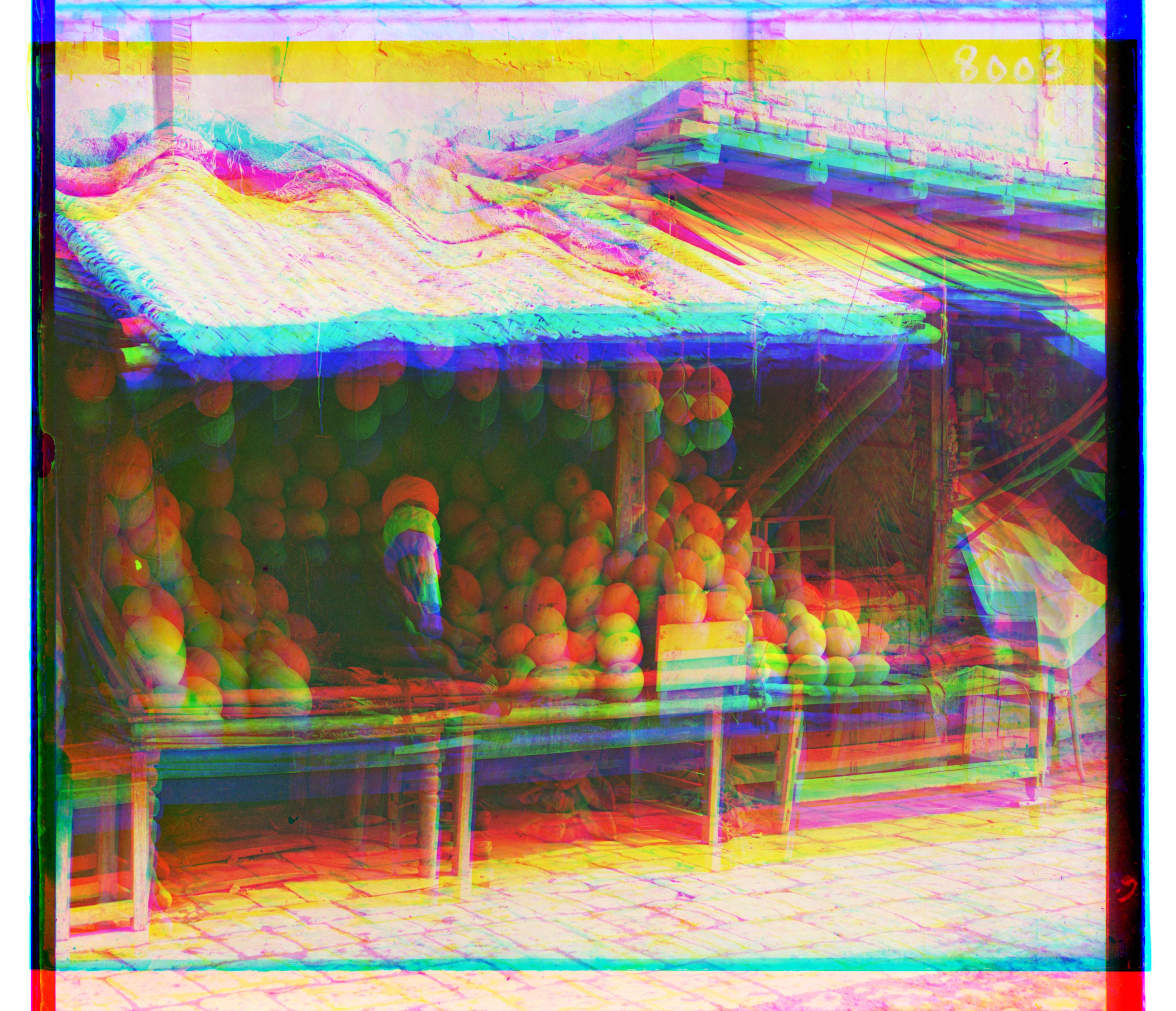
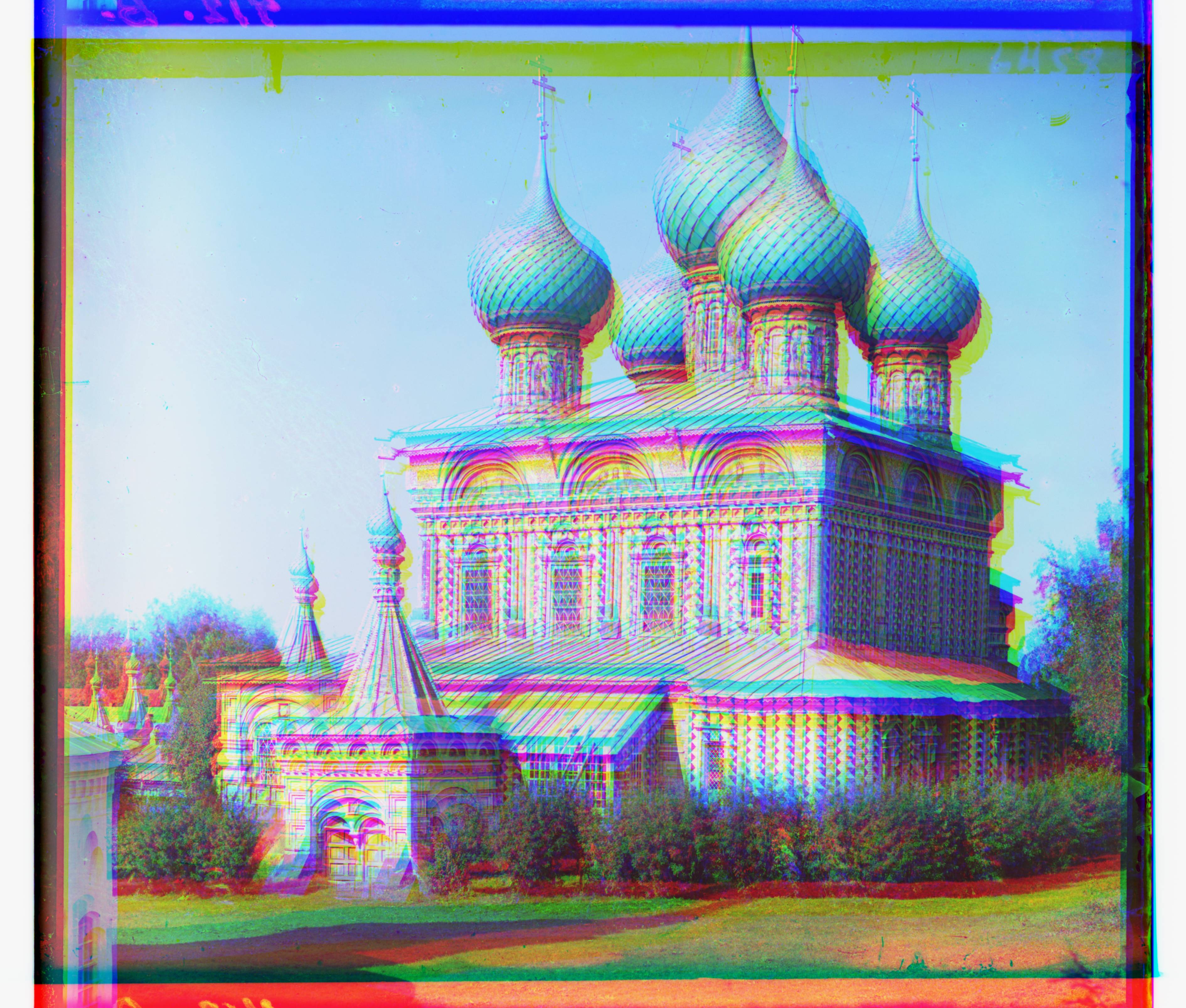
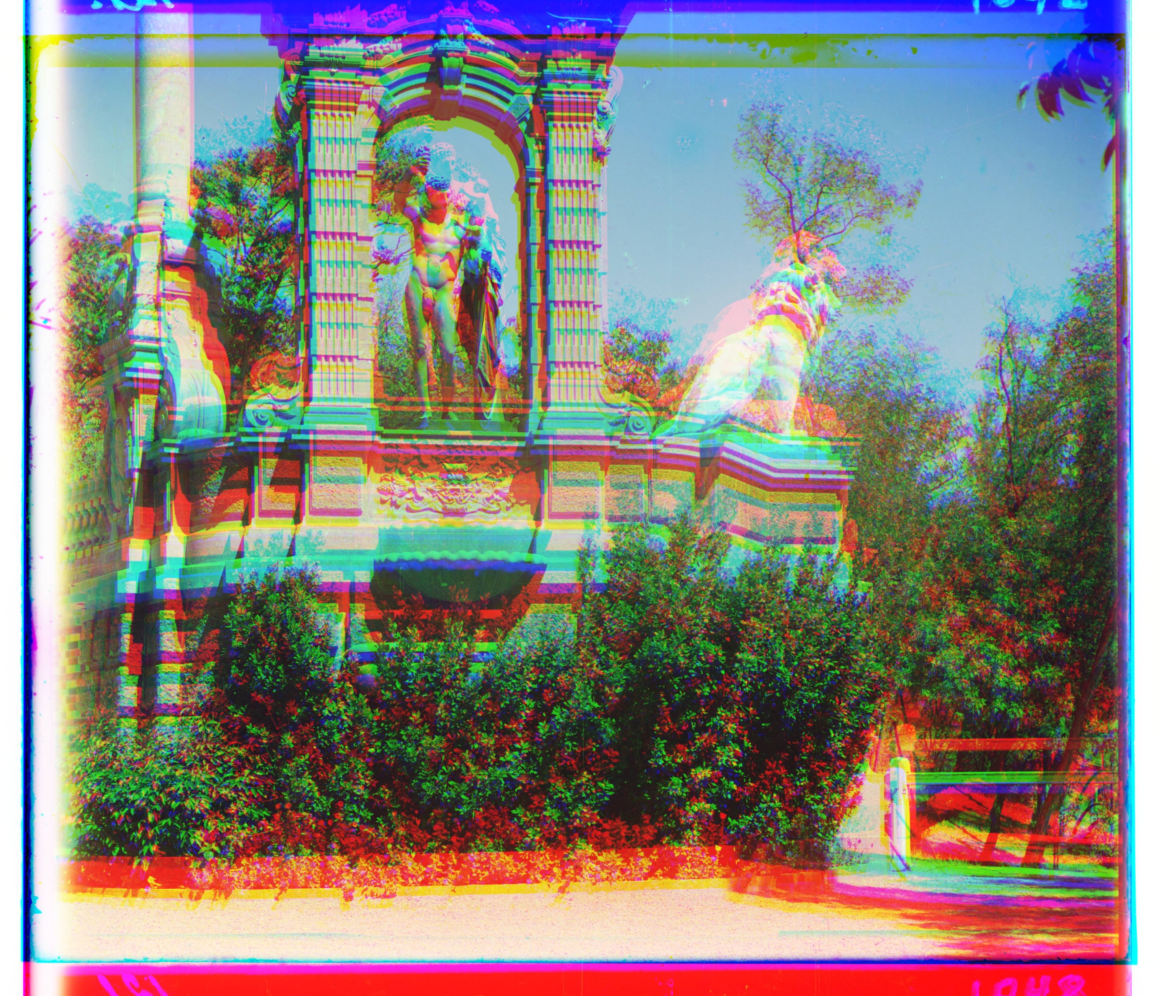
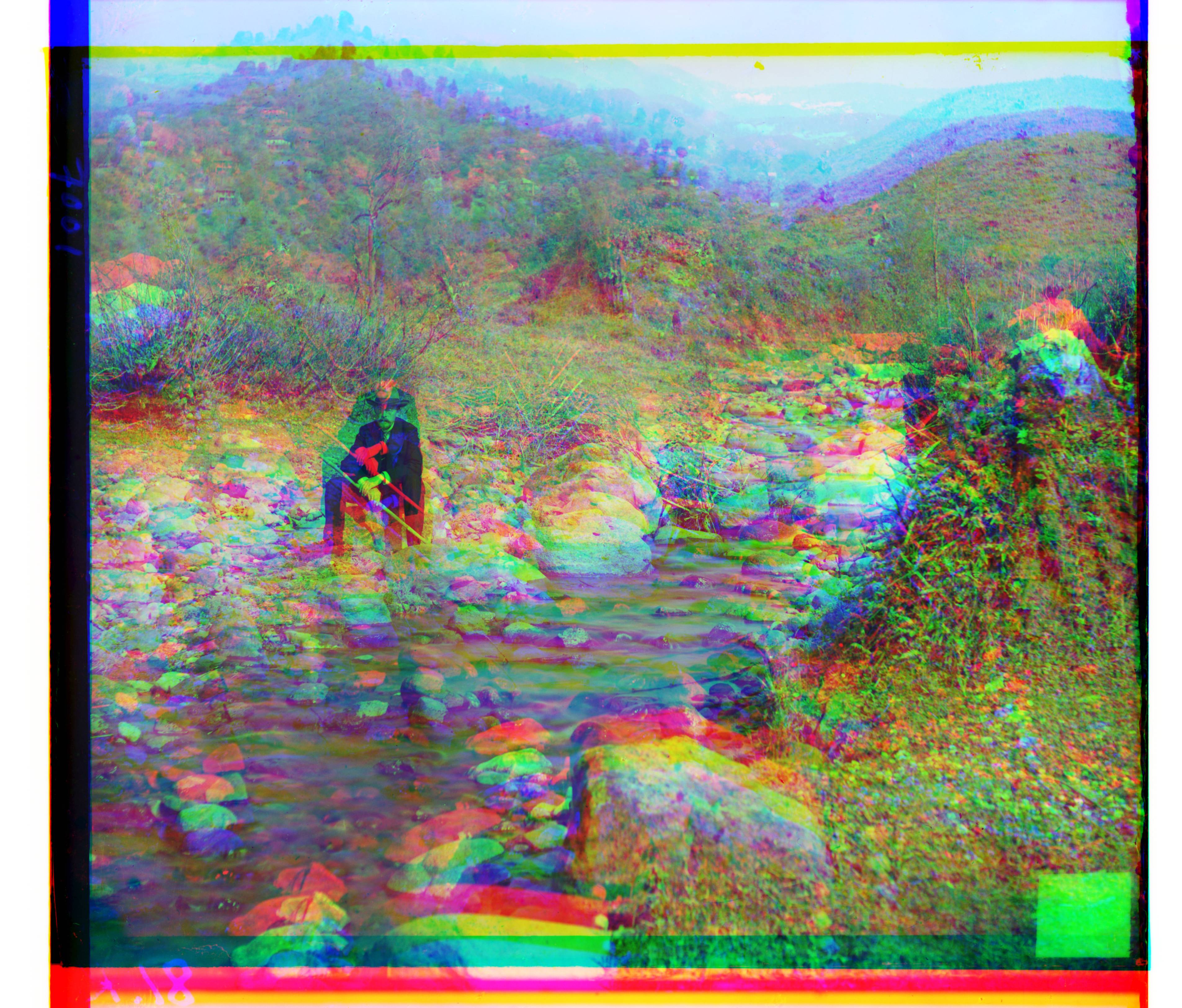
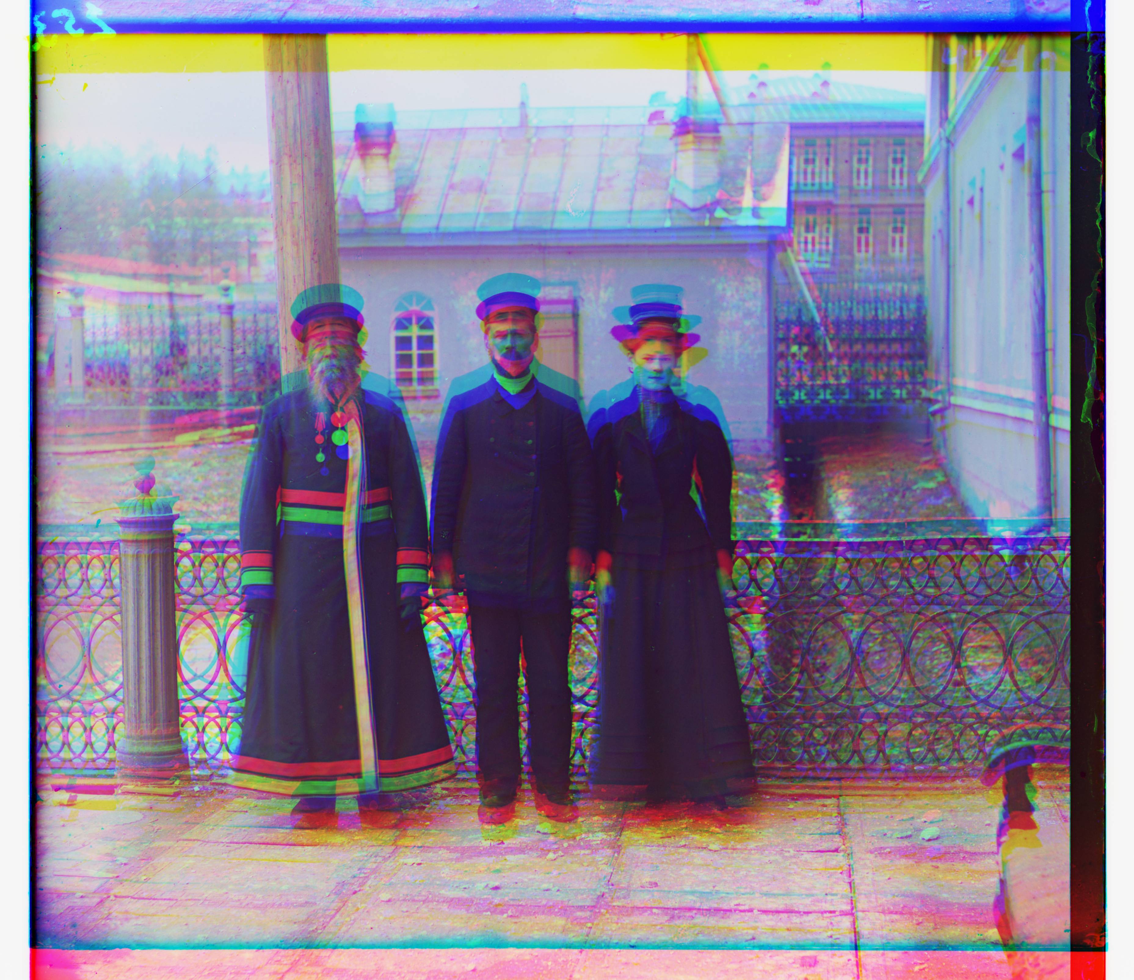
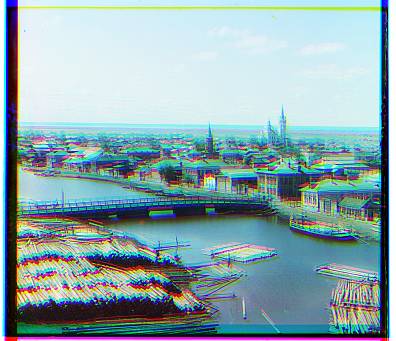
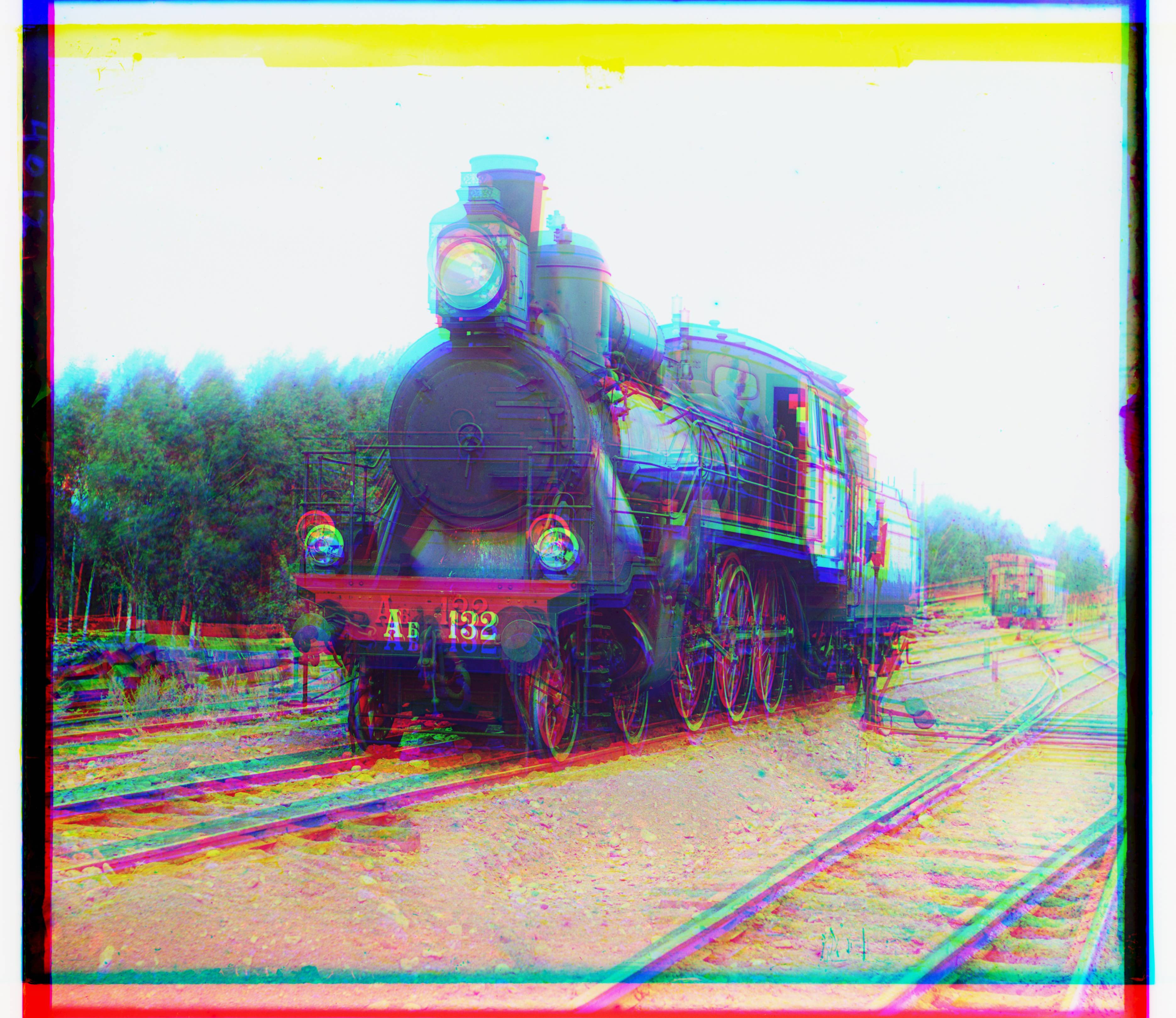
As we can see, the naive approach performs very poorly. Due to the mis-alignment of the images, the produced color image is not an accurate depiction of Prokudin-Gorskii’s intended image.

Single Scale Alignment

The first approach I took towards aligning the images was to use a relatively simple and brute force approach, sliding the image over each other to compare the similarity. I allowed maximum displacements of 15 px of each dimension, allowing for some leeway given that images were not perfectly square. I fixed the blue channel and aligned the green and red channels. This resulted in displacement vectors for the green and red channels that I could use to produce an aligned image.

Alignment Metric

While sliding the images over each other, it may be easy for a human to tell when they are aligned, however, it is not so trivial for a computer. To align our images we need to have a metric to quantify the alignment of the images. The one that I settled upon was the Normalized Dot Product.

Where \(\|A\|\) and \(\|B\|\) are the magnitudes of the vectors and \(\theta\) is the angle between them. The normalized dot product is defined as:

With some algebra, we can see that the normalized dot product is equal to the cosine similarity between the two vectors. The cosine similarity is a measure of similarity between two non-zero vectors of an inner product space. The cosine of 0 degrees is 1, and decreases for any other angle. Thus we have our metric, where the closer the normalized dot product is to 1, the more “aligned” we believe the images to be.

However, at the resolutions where a single scale level approach is reasonable (the search space increases exponentially as the image grows), I found that often using a metric such as the Normalized Dot Product or Mean Squared Error was not enough to accurately align the images. The images would often be content with 0,0 displacement. As such, I decided to use an extracted feature from the images to align them.

Alignment Heuristic

I settled on using image edges as the feature to align the images. While I originally developed my own rudimentary edge detector by traversing the image top to bottom and left to right, and noting changes over a threshold, and merging them with a logical or, the custom edge detection was both slow and unreliable for larger images. I used the Canny edge detector to extract the edges from the images.

Before extracting the edges from our image, it is important to note that because our images are noisy, this can greatly hamper the output of our edge detection.

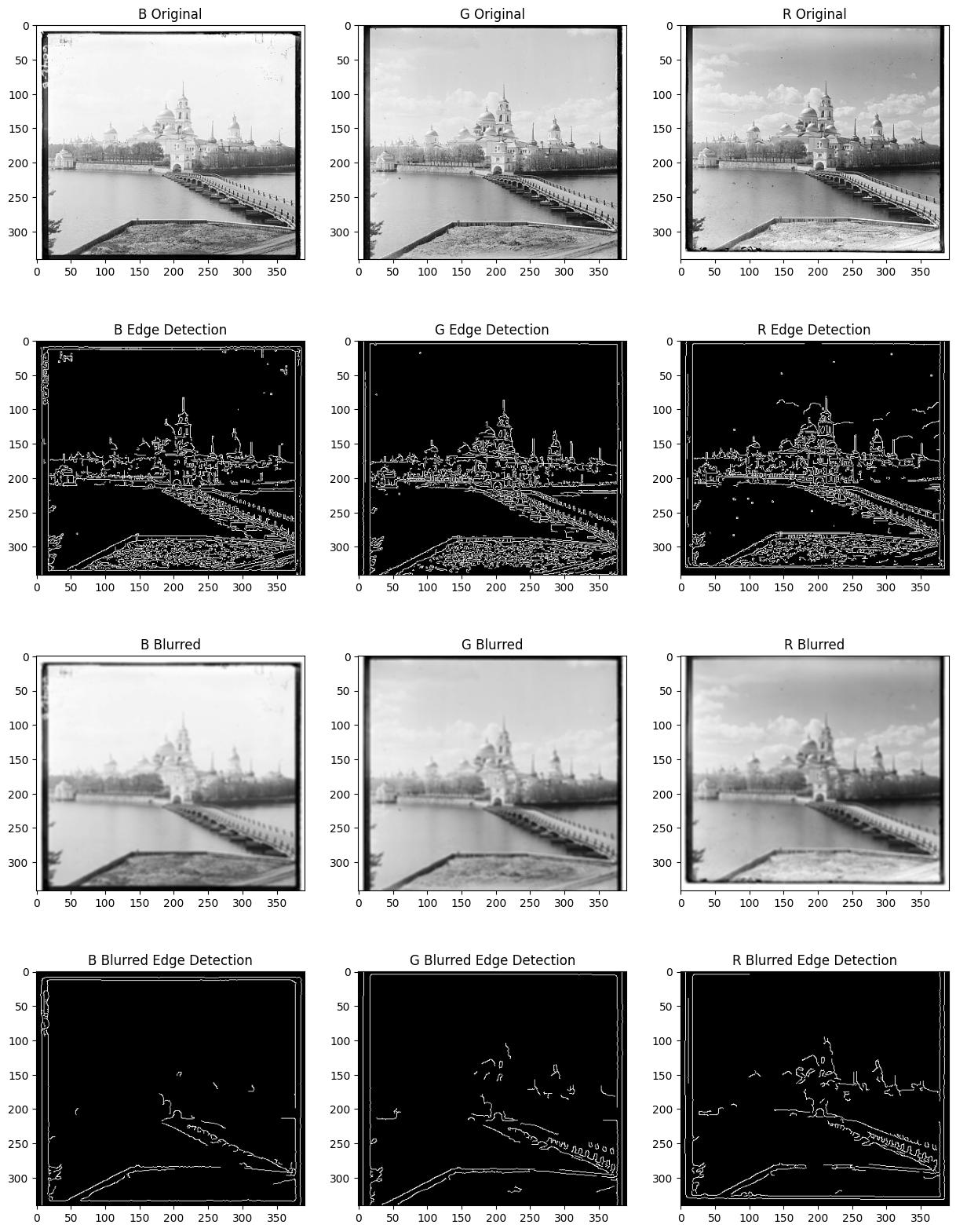
Lastly, because the border of Prokudin-Gorskii’s images are white and then black, the edge detection produces very strong lines that are not affected by the Gaussian blurring. These lines are not features that we want to consider in aligning our image because the border does not correspond to the actual alignment of the image. Therefore, we take a 15% crop on all sides of the channel, removing the border and any defects that may have arisen from the border intruding into the exposure.

Conclusion

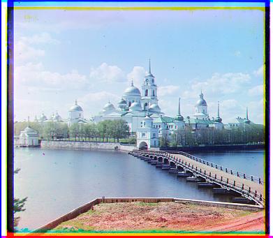
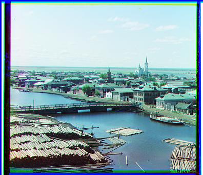
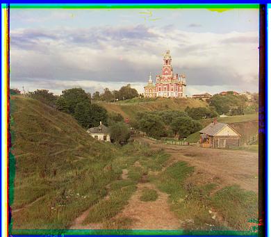
Our final result processes the JPEGs from Prokudin-Gorskii’s collection in a matter of seconds. I am using the common image coordinate system, where the origin is at the top left corner of the image, the x-axis is positive to the right, and the y-axis is positive downwards. The dY, and dX values are the displacements in the y and x directions respectively.

Examples

Multi-Scale Alignment

We will now be dealing with much larger images, where each channel’s dimensions are around 3 thousand pixels. A 10% displacement in each direction would result in a search space of 300 by 300 pixels. This 90,000 pixel search space is not feasible to search through, and as such we will be using a multi-scale approach to align our images.

Gaussian Pyramids

To represent images are lower resolutions, we will be using Gaussian Pyramids. A Gaussian Pyramid is a collection of images, where each image is a smoothed and downscaled version of the image below it. The bottom of the pyramid is the original image, and the top of the pyramid is the smallest image, as such the pyramid consists of layers. By convention, the original image is the 0th layer, and the smallest image is the \(k\)th layer.

Formula for Maximum Displacement

We can make some observations at this point. Because at each layer our displacement from the layer above doubles, there must be an optimal displacement range such that we can attain a large alignment precision. At layer \(k\), a single pixel shift corresponds to a shift of \(2^k\) pixels in the original image. Our maximum displacement can be considered another value, let’s use \(r\), and the area we are trying to cover, in our earlier example 15%, can become \(p\). Additionally, let us consider our highest layer to be \(L\). \(n\) is the number of pixels in the dimension we are trying to align.

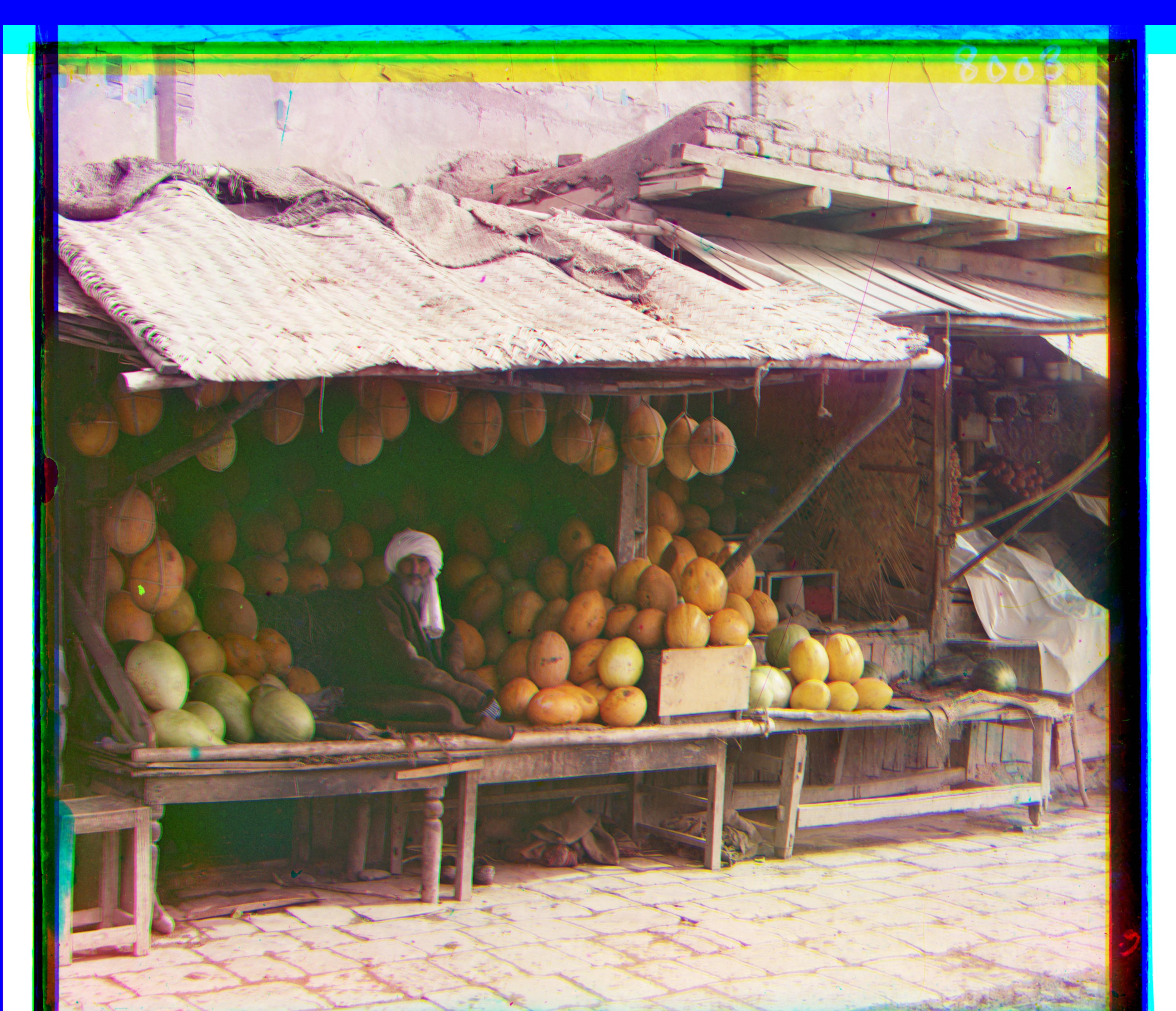
Now that we have a formula for our maximum displacement, we must decide on fixing the variables \(p\) and \(L\). Upon rounds of testing, and specific increases to allow for the alignment of melons, I settled on \(p\) to be 10%. Because \(r\) decreases as \(L\) increases, a higher \(L\) will allow for a faster alignment, as there will be more layers, but the search space in each will be smaller. This is trading the exponential growth of the search space for the linear growth of the number of layers. However, as L increases, the resolution of the image decreases, and the edge heuristics become less reliable. I settled on computing and choosing an \(L\) such that the smallest dimension of the image at layer \(L\) is ~50 pixels.

This method was shared with the single scale alignment, however, because there are 0 layers, it increased the search space to 10% of the level 0 image, usually around 300 pixels. This resulted in slightly higher computation times than before, but still on the order of seconds, so the times above are from this version.

Conclusion

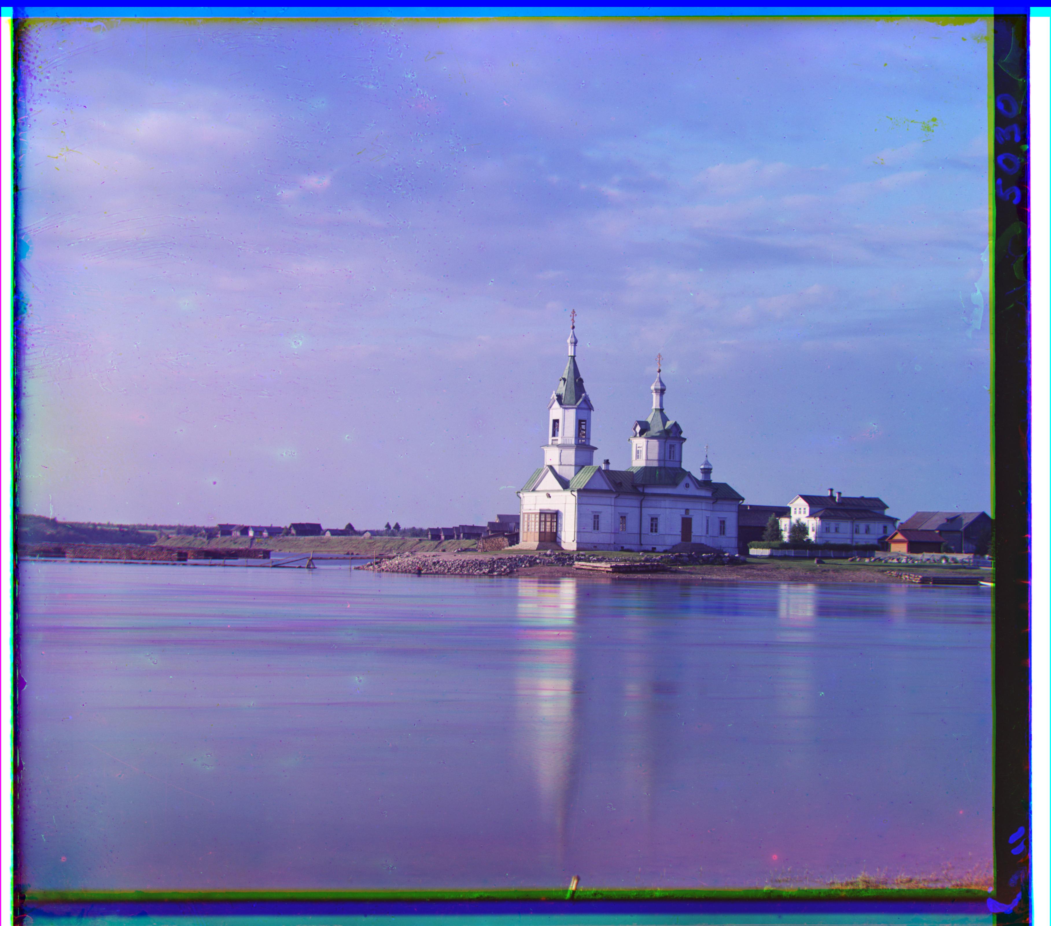
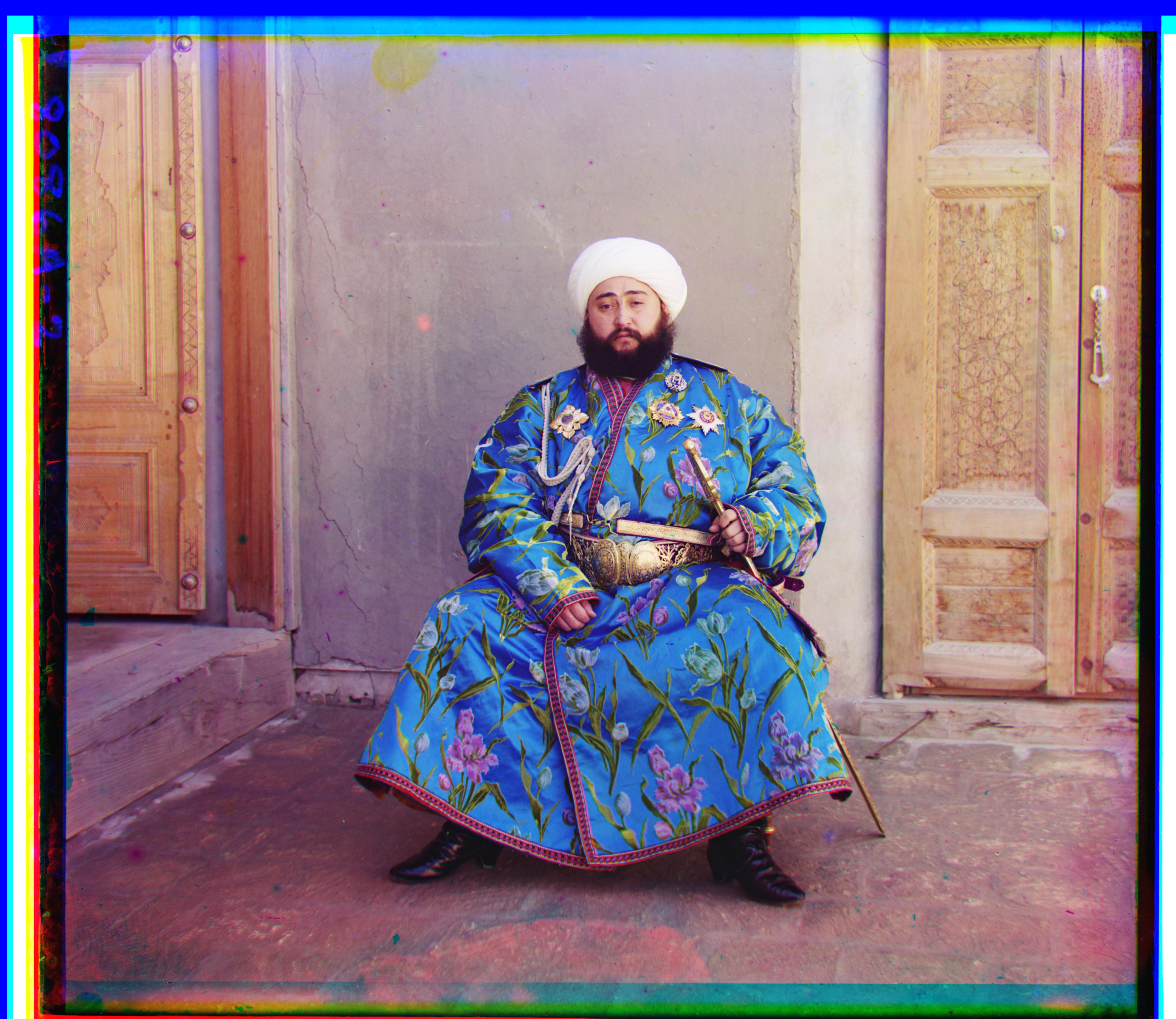
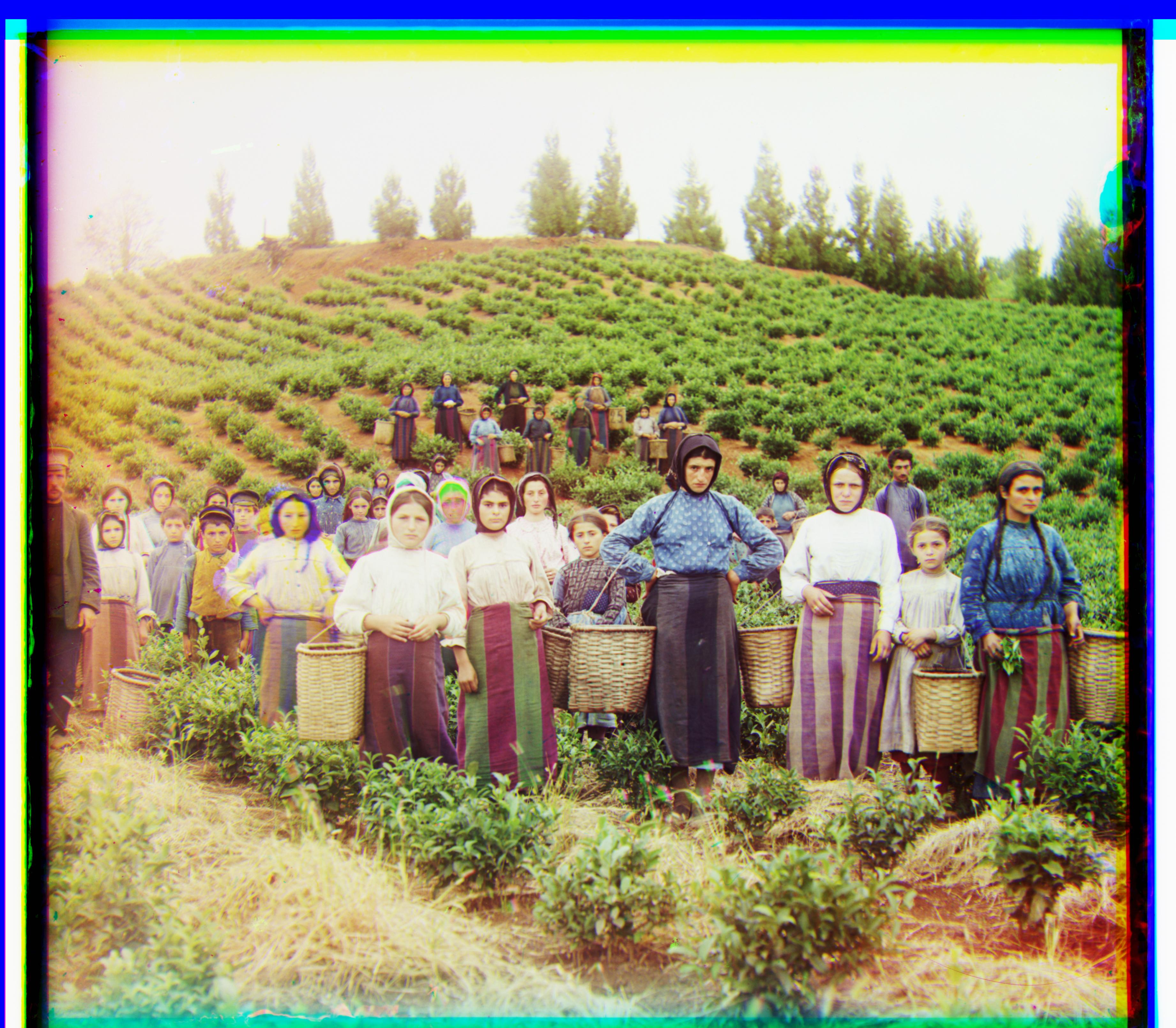
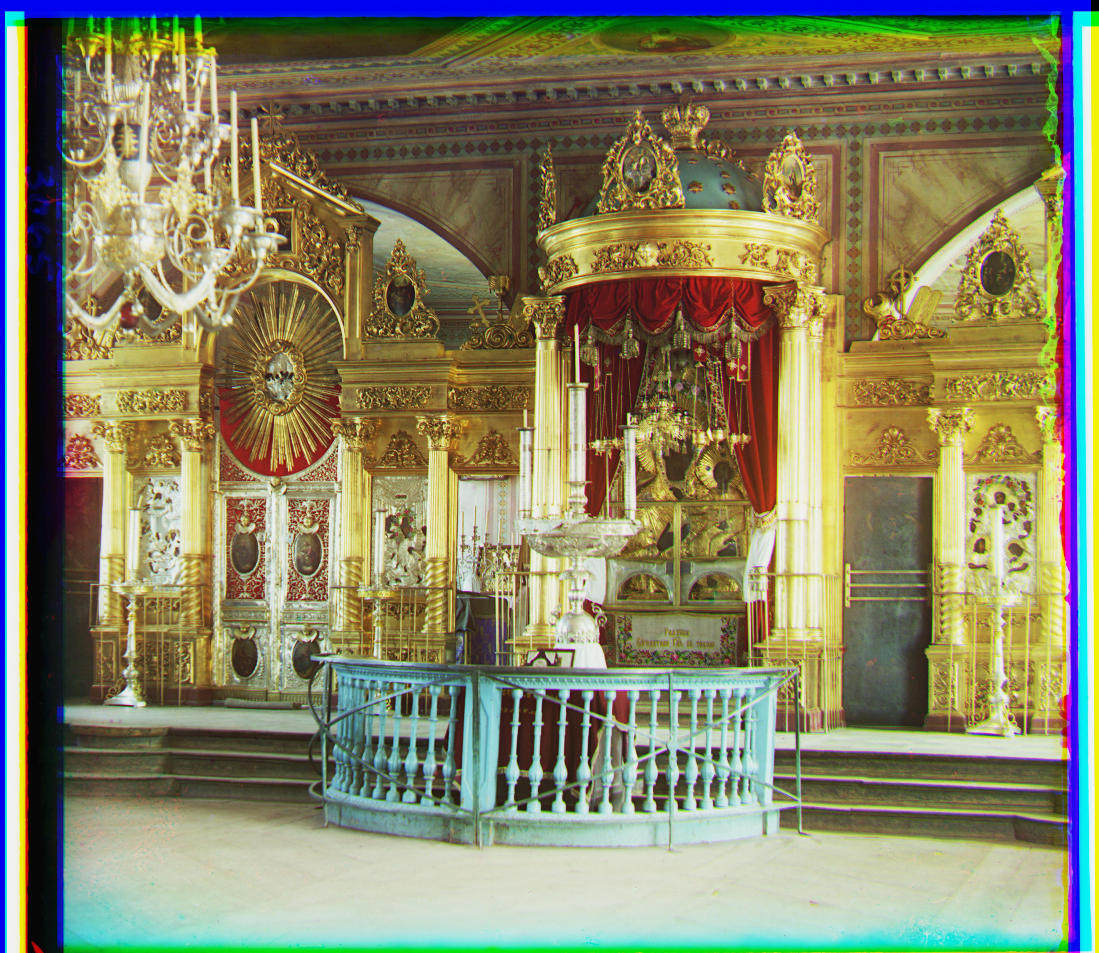
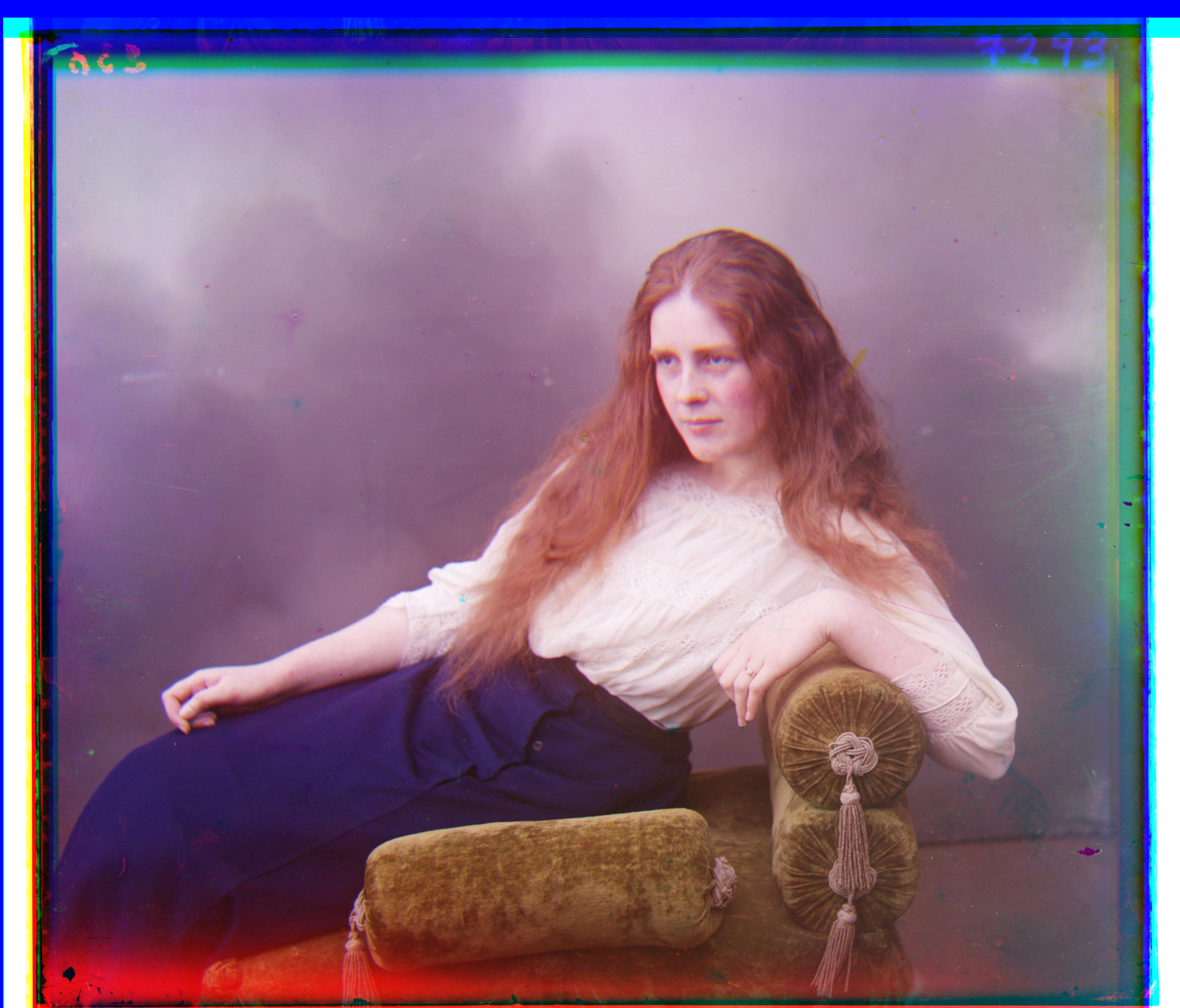
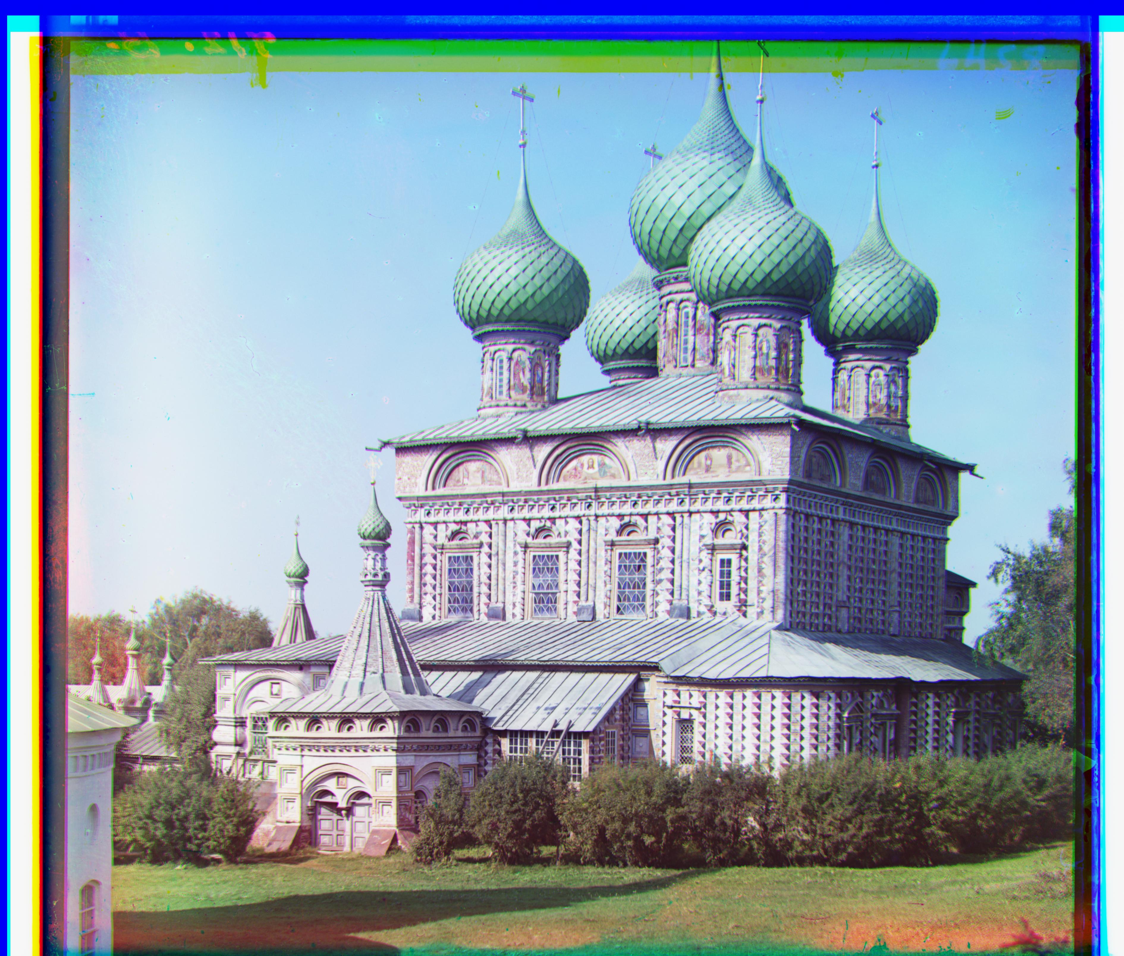
The multi-scale alignment approach is able to align the images with a high degree of accuracy and with incredible speed! The images are aligned in a matter of seconds, and the results are quite impressive. While using a fixed L of 5, the tiff images took on the order of 4 minutes to complete alignment at level 0. However, with a variable L, the images are aligned in a matter of seconds.

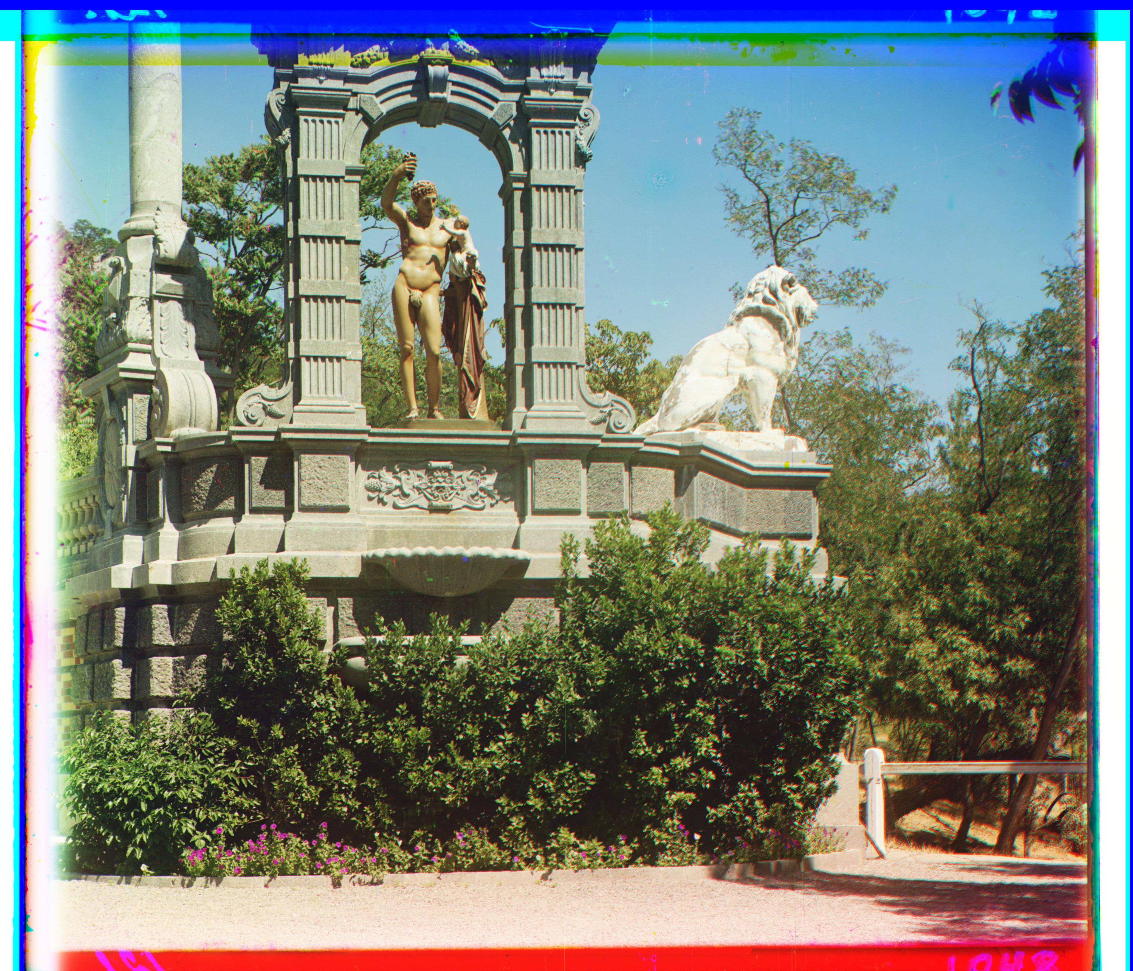
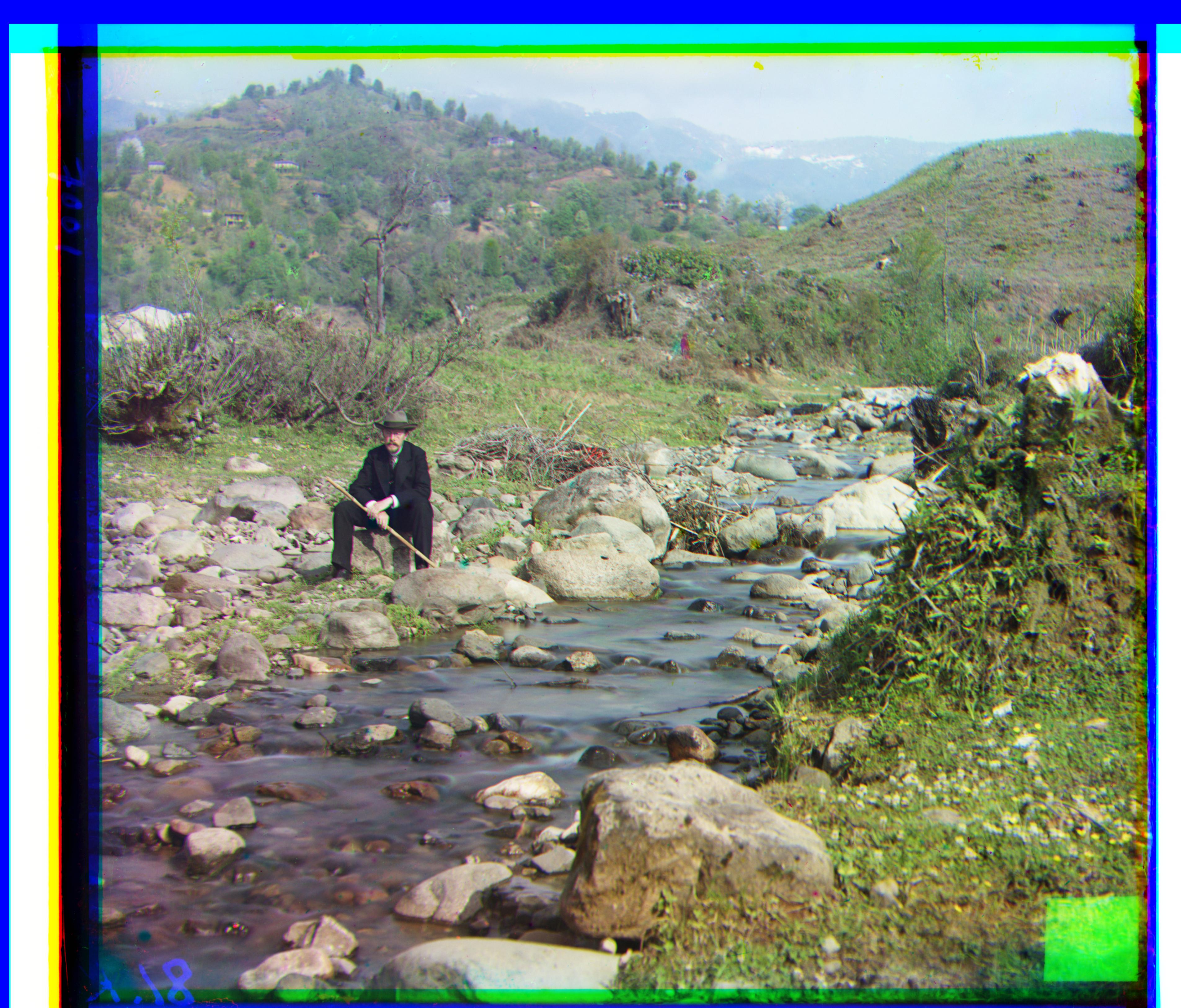
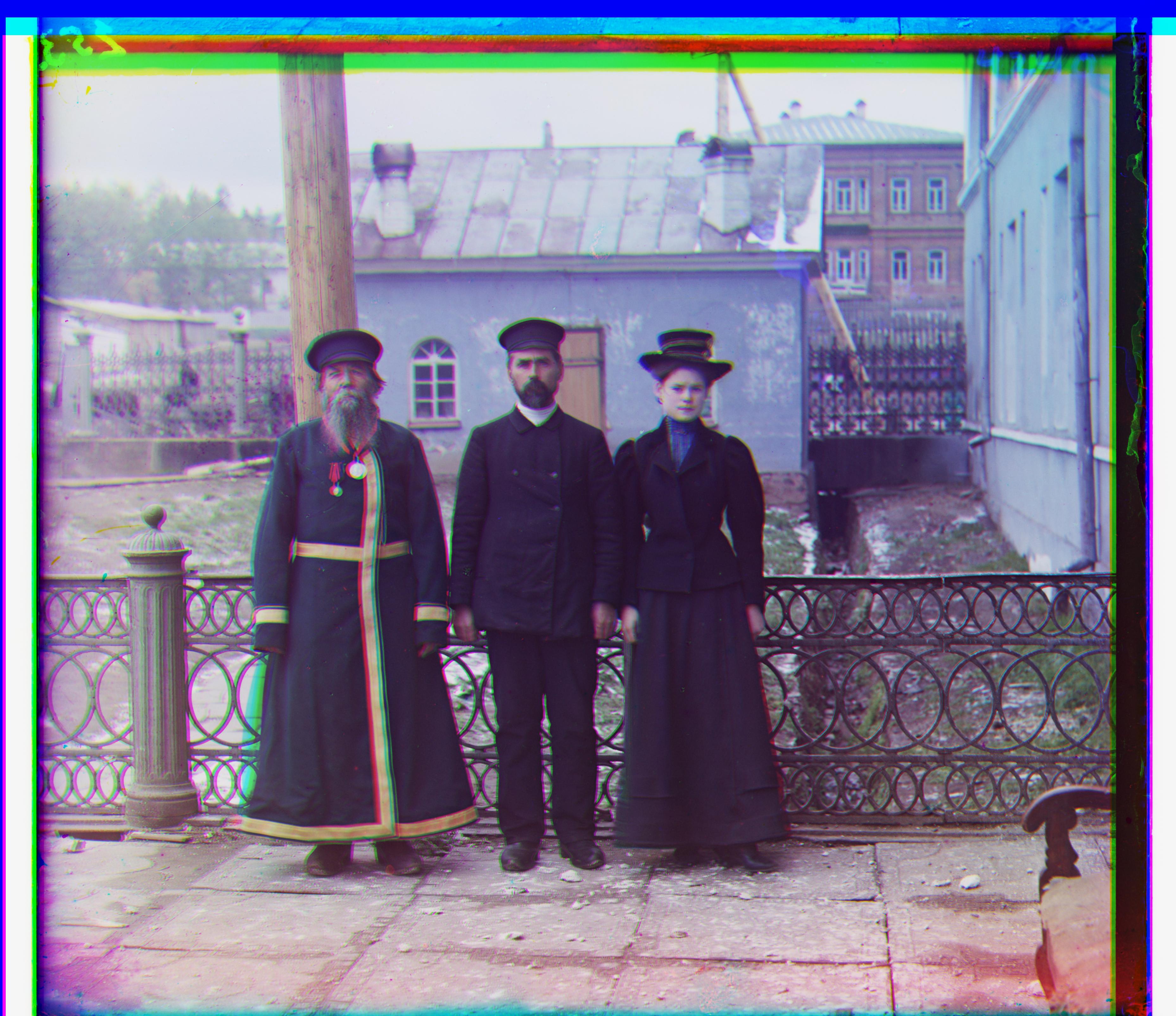
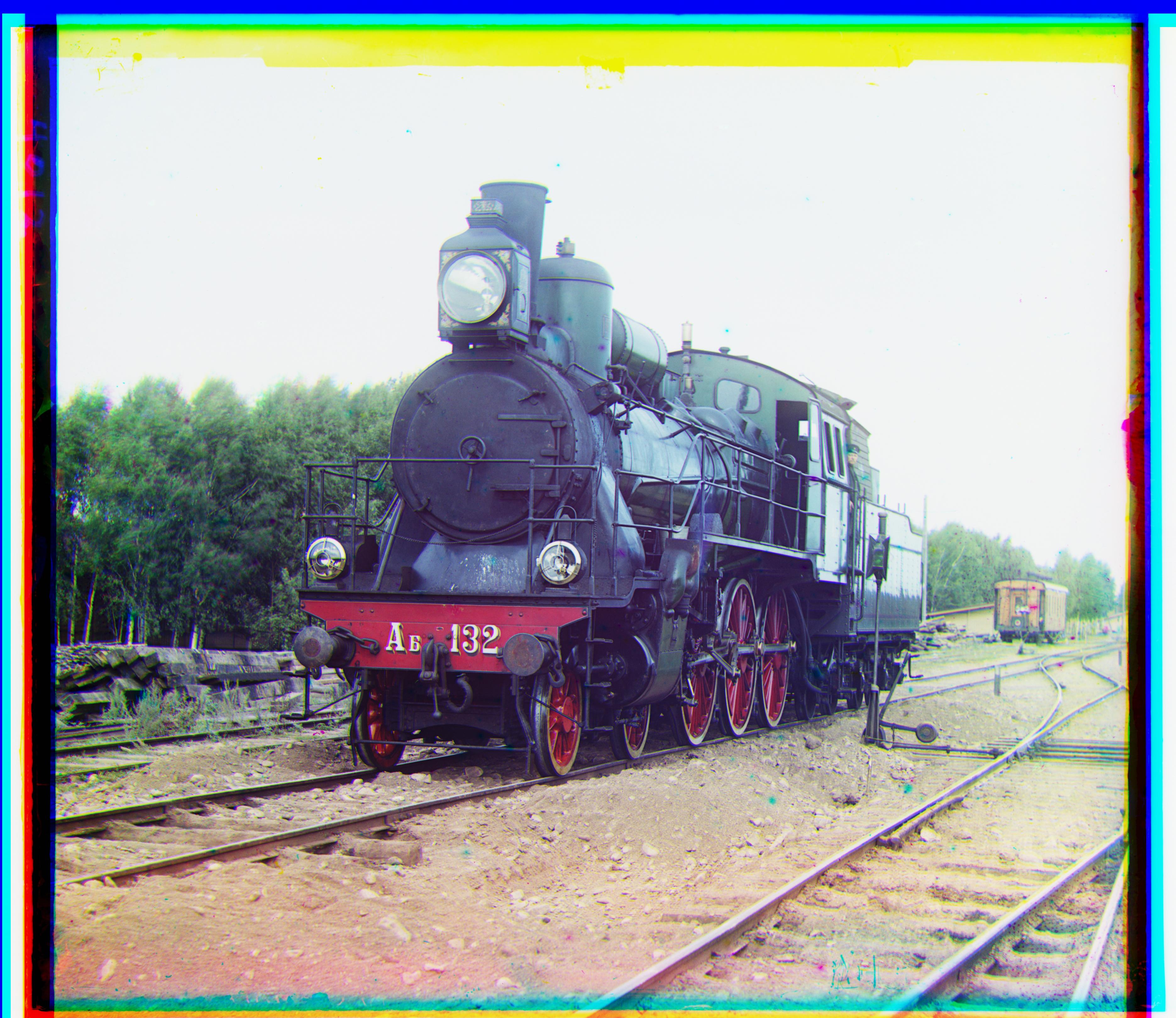
Examples

Side Notes

Some other ideas I tried included using phase-based correlation to align the images, however after refactoring my code, I found that the function was no longer working. Regardless, I was able to verify the accuracy of my alignment using sci-kit image’s phase-based correlation method and found that my alignment agreed well with the results of the phase-based correlation. This satisfied me with the knowledge that my methodology was validated by fft frequency correlation.a