Cloth Simulation
Part of CS184 : Foundations of Computer Graphics
https://satish.dev/projects/homework_4
Overview
In this assignment, I implemented a cloth simulation using a mass-spring system. The cloth is represented as a grid of point masses connected by springs, which allows for realistic deformation and movement. The simulation uses numerical integration to update the positions and velocities of the point masses over time. I also implemented collision detection and response with other objects, such as spheres and planes, as well as self-collision handling to prevent the cloth from passing through itself. I learned a lot about the intricacies of simulating physical systems, including the challenges of maintaining stability and realism in the simulation. I also gained experience in implementing shaders for rendering the cloth, which added a new layer of complexity to the project. I had a lot of fun exploring creative ways to color the scene in the custom shading section, and I ended up learning a lot about shaders! Overall, this assignment was a valuable learning experience that deepened my understanding of computer graphics and physics-based simulations.
Masses and Springs
In this part, I implemented a mass-spring system to represent the cloth. The cloth is made up of point masses connected by springs, which represent the cloth’s elements of structure, bending, and shearing.
The point masses are arranged in a grid, and each point mass is connected to its neighbors by springs. The springs have a rest length, which is the length of the spring when it is not under any force. There are three types of springs in the simulation: structural springs, shearing springs, and bending springs.
Structural springs connect point masses that are adjacent in the grid, they are responsible for maintaining the overall shape of the cloth. Shearing springs connect point masses that are diagonally adjacent in the grid, they are responsible for maintaining the cloth’s shear resistance. Bending springs connect point masses that are two units apart in the grid, they are responsible for maintaining the cloth’s bending resistance, which allows the cloth to bend and fold realistically, however this force is weaker than the other two forces.
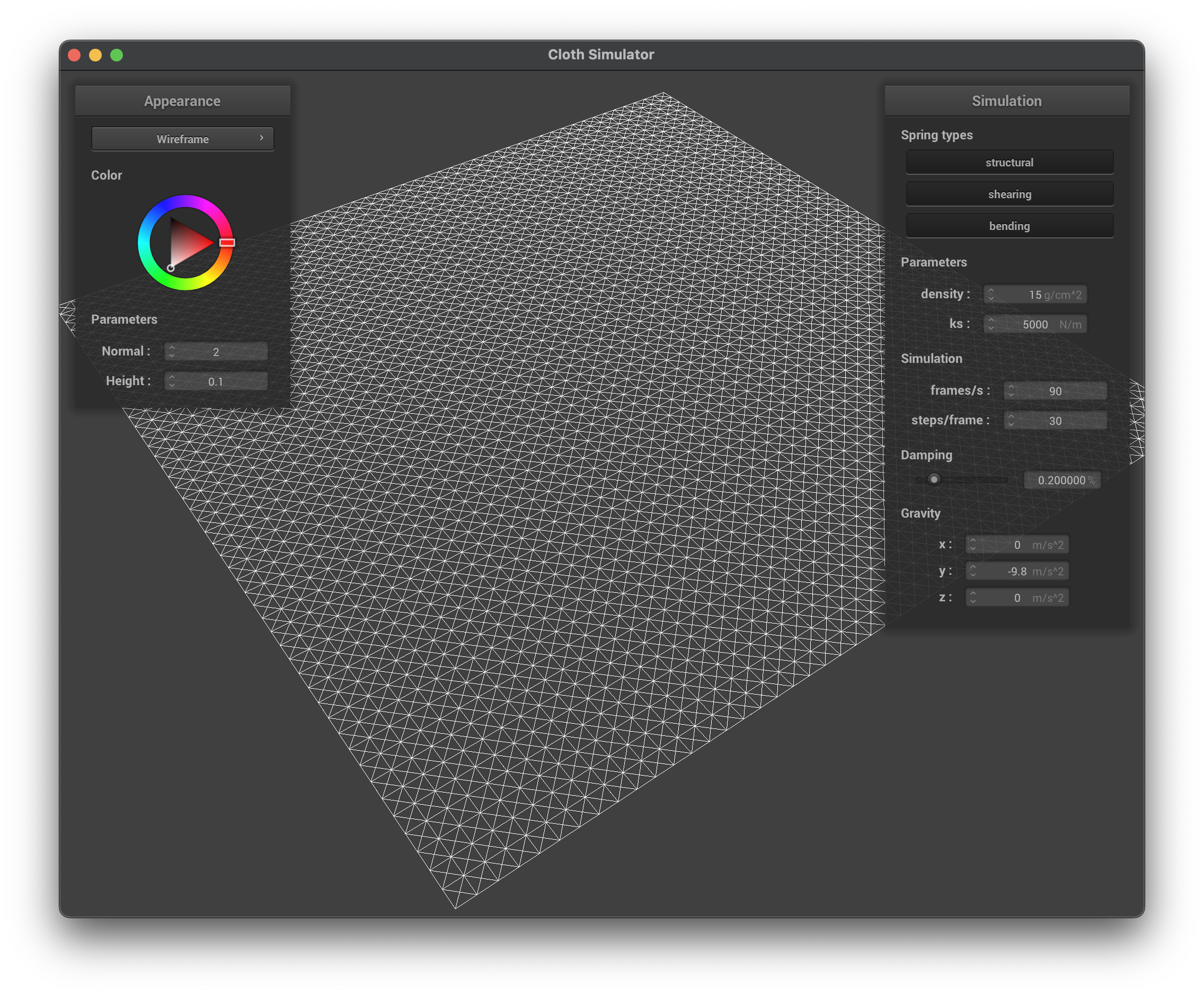
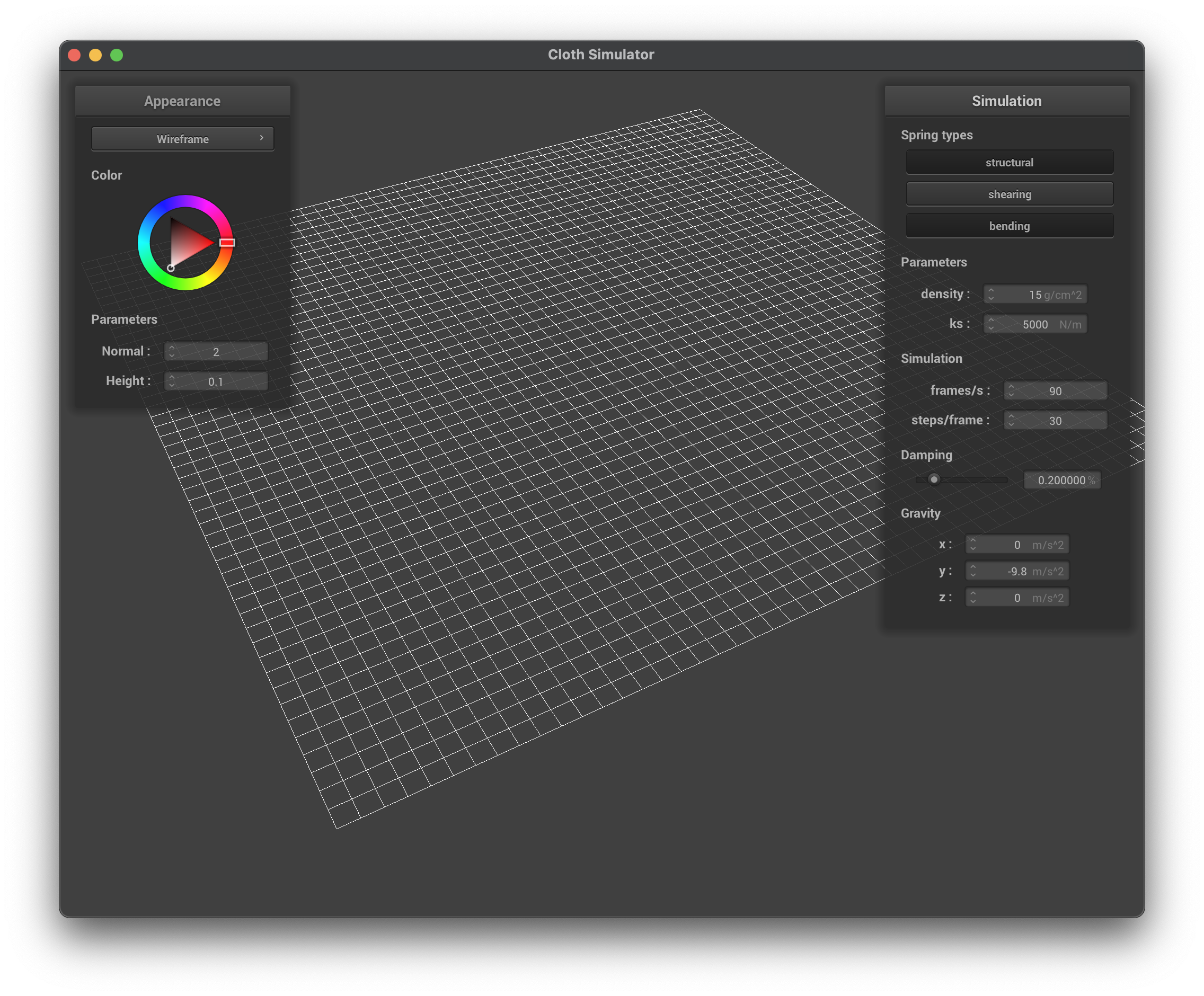
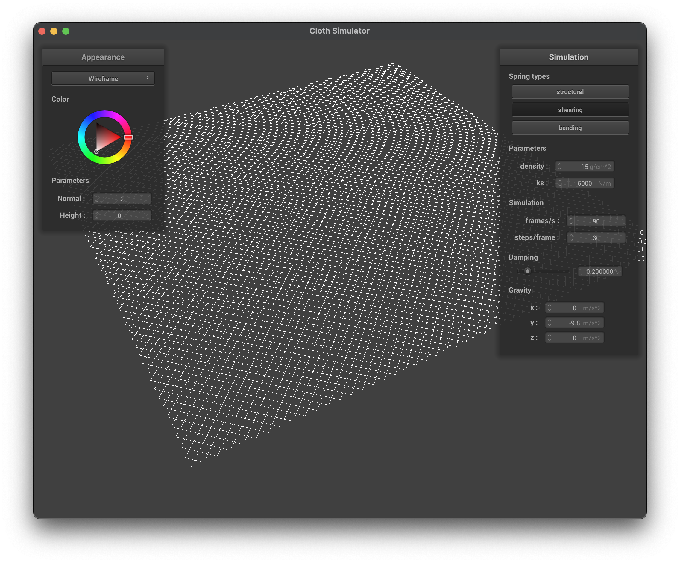
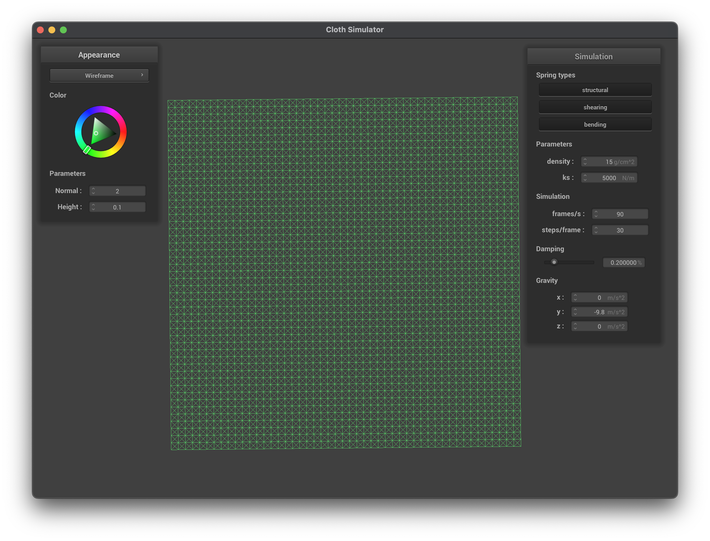
The first image shows the wireframe of the cloth at an angle where the structure of the point masses and springs is clearly visible. The third image shows the wireframe without any shearing constraints, which is an x-y grid of point masses connected by springs. The fourth image shows the wireframe with only shearing constraints, this is where the diagonal springs are added to the grid. The fifth image shows the wireframe with all constraints, including the bending and shearing constraints.
Simulation via Numerical Integration
In this part, I implemented the simulation of the cloth using numerical integration. We begin by applying the external forces to the point masses, such as gravity and any other user-defined forces. Next, we compute the forces acting on each point mass based on the spring forces. To do so, we utilize Hooke’s law, which states that the force exerted by a spring is proportional to its displacement from its rest length.
\[F\_{spring} = -k_s \cdot (x - x_0)\]where \(F\_{spring}\) is the spring force, \(k_s\) is the spring constant, \(x\) is the current length of the spring, and \(x_0\) is the rest length of the spring.
We then apply the forces to the point masses and update their positions and velocities using Verlet integration. The Verlet integration algorithm is a numerical method used to integrate Newton’s equations of motion. It is particularly well-suited for simulating physical systems, as it conserves energy and momentum better than other methods. The Verlet integration algorithm consists of two main steps: updating the positions and updating the velocities. The position update is done using the following equation: \(x_i(t + \Delta t) = x_i(t) + v_i(t) \cdot \Delta t + \frac{1}{2} a_i(t) \cdot (\Delta t)^2\)
where \(x\_i\) is the position of the point mass, \(v_i\) is the velocity, \(a_i\) is the acceleration, and \(\Delta t\) is the time step. However, in Verlet integration, we utilize the estimation that \(v_i(t) \cdot \Delta t\) is equal to \(x_i(t) - x_i(t - \Delta t)\), which allows us to update the position without explicitly calculating the velocity. The acceleration is calculated based on the forces acting on the point mass: \(a_i(t) = \frac{F_i(t)}{m_i}\)
This method allows for an accurate simulation of the cloth’s motion and deformation, while maintaining stability and energy conservation. However, because in real life we lose energy due to friction, noise, etc., we need to add a damping factor to the simulation. The damping factor is a constant that reduces the velocity of the point masses over time, simulating the loss of energy in the system. The damping factor is applied to the velocity update equation:
//pm.position + (1 - cp->damping/100) _ (pm.position - pm.last_position) + (pm.forces / mass) _ delta_t * delta_t;
\[x_i(t + \Delta t) = x_i(t) + (1 - d) \cdot (x_i(t) - x_i(t - \Delta t)) + \frac{1}{2} a_i(t) \cdot (\Delta t)^2\]where \(d\) is the damping factor. This equation allows us to simulate the loss of energy in the system, resulting in a more realistic simulation of the cloth’s motion.
Results
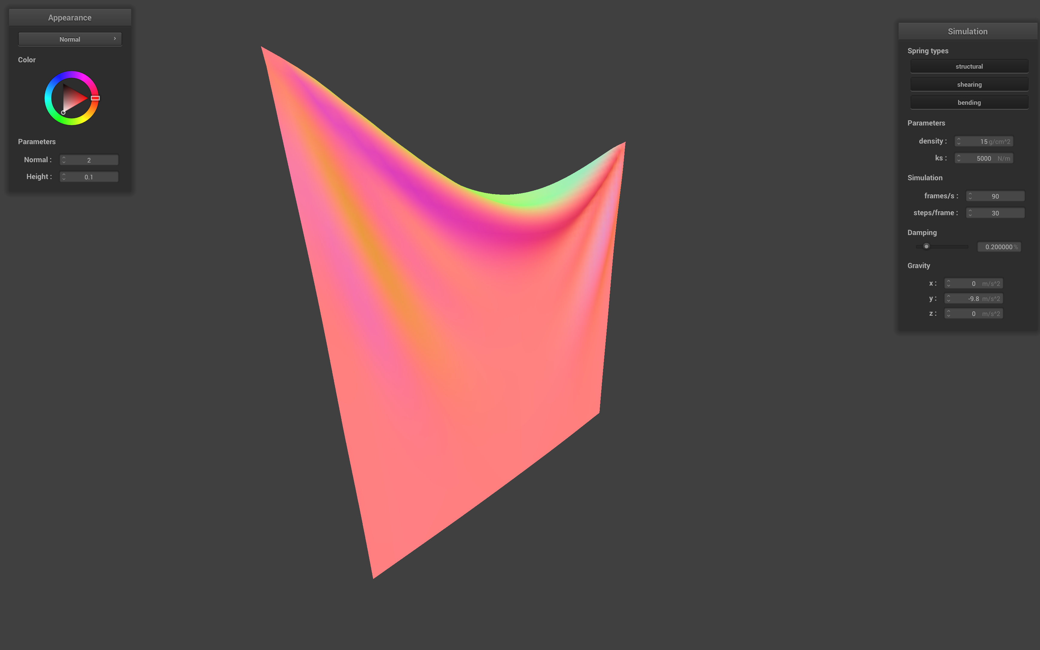
The first image shows the default rest state of the cloth. The second row shows the default simulation, double density simulation, and half density simulation. The third row shows the default simulation with 3 directional acceleration (3,-9.8,3), double spring constant simulation, and half spring constant simulation. The fourth row shows the zero damping simulation, 1% damping simulation, and 10% damping simulation. The fifth row shows the 50% damping simulation and 100% damping simulation.
I made the following observations:
- Spring Constant (ks): Increasing the spring constant results in a stiffer cloth that resists deformation, notably bending, more, while decreasing it results in a more floppy cloth that has more ripples.
- Density: Increasing the density results in a heavier cloth that falls faster and has more inertia, while decreasing it results in a lighter cloth that falls slower and has less inertia. The stretch applied at rest is also more pronounced with a higher density.
- Damping: Increasing the damping factor results in a cloth that loses energy more quickly and comes to rest faster, while decreasing it results in a cloth that retains energy longer and bounces more. The damping factor also affects the stability of the simulation, with higher values resulting in a more stable simulation. At 0% damping, the cloth oscillates indefinitely, while at 100% damping it seems like it is a linear interpolation between the start and end positions.
Handling Collisions with Other Objects
In this part, I implemented collision detection and response with spheres and planes. The collision detection algorithm checks if the point masses are colliding with any collision objects, such as spheres or planes, in the scene and updates their positions to prevent them from rendering inside the objects.
Sphere Collision
In the sphere collision detection algorithm, I calculate the distance between the point mass and the center of the sphere. If the distance is less than the radius of the sphere, I calculate the normal vector from the center of the sphere to the point mass and normalize it. I then calculate the tangent point on the surface of the sphere and apply a correction to the position of the point mass to prevent it from penetrating the sphere. The correction is scaled by a friction factor to allow for some sliding along the surface of the sphere.
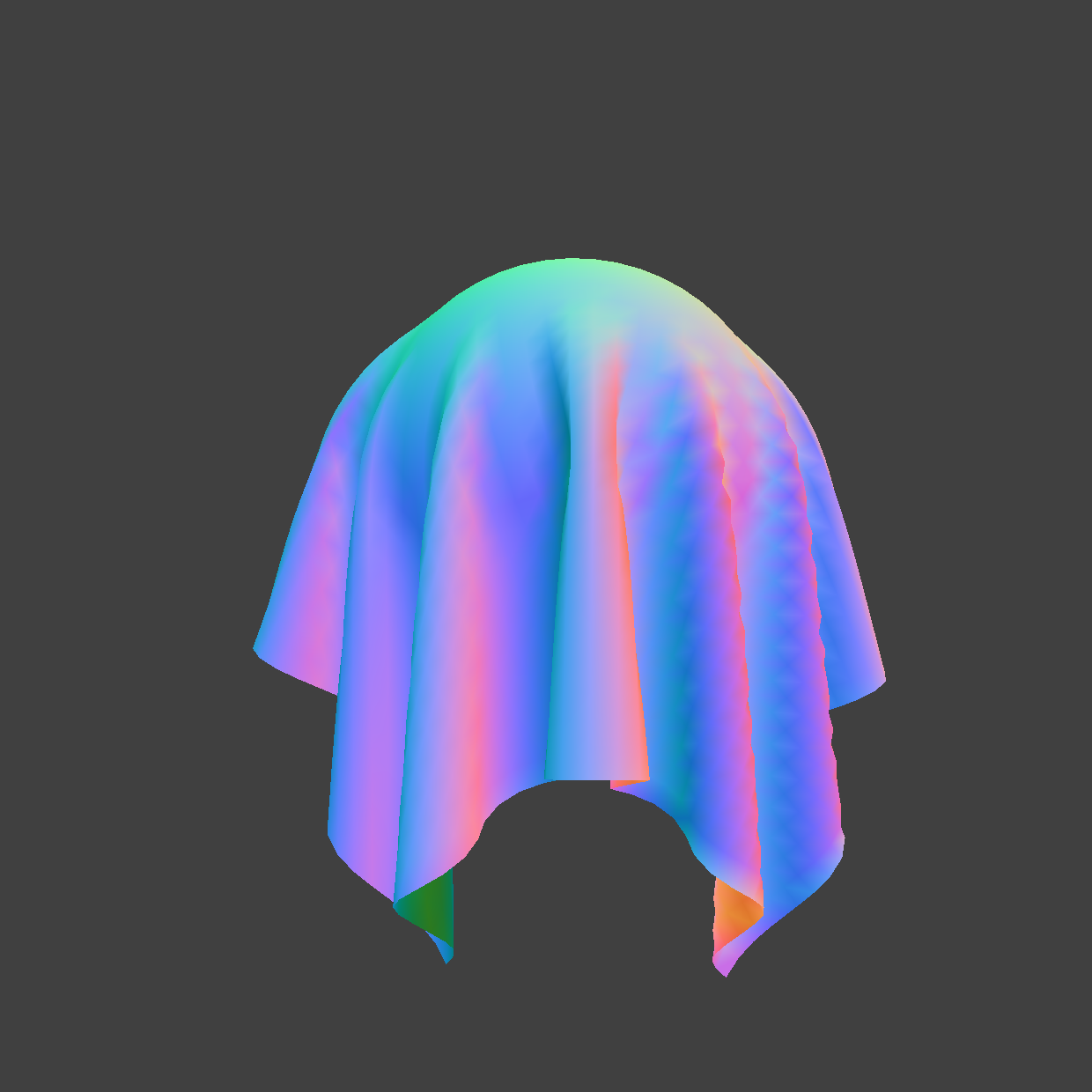
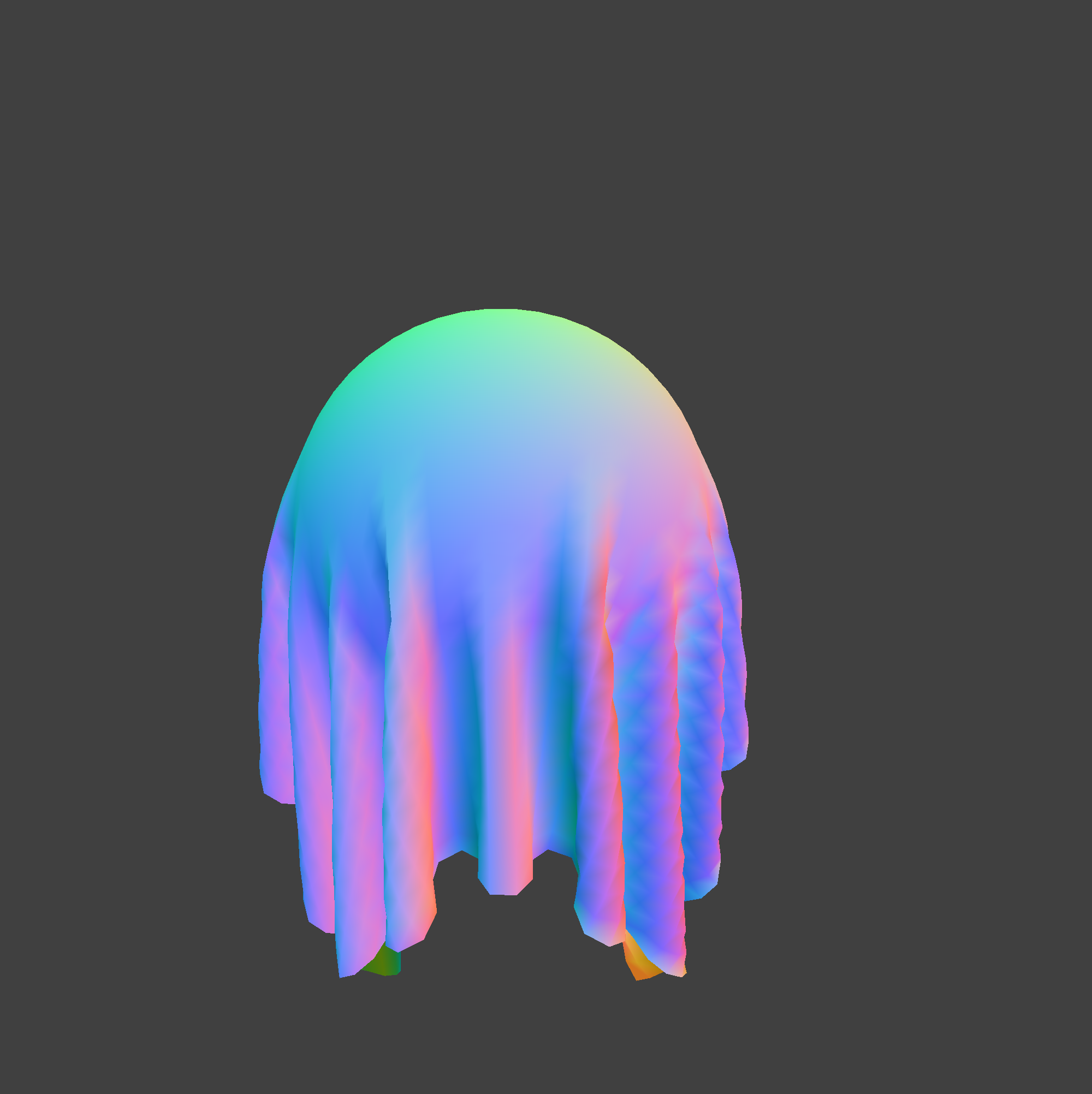
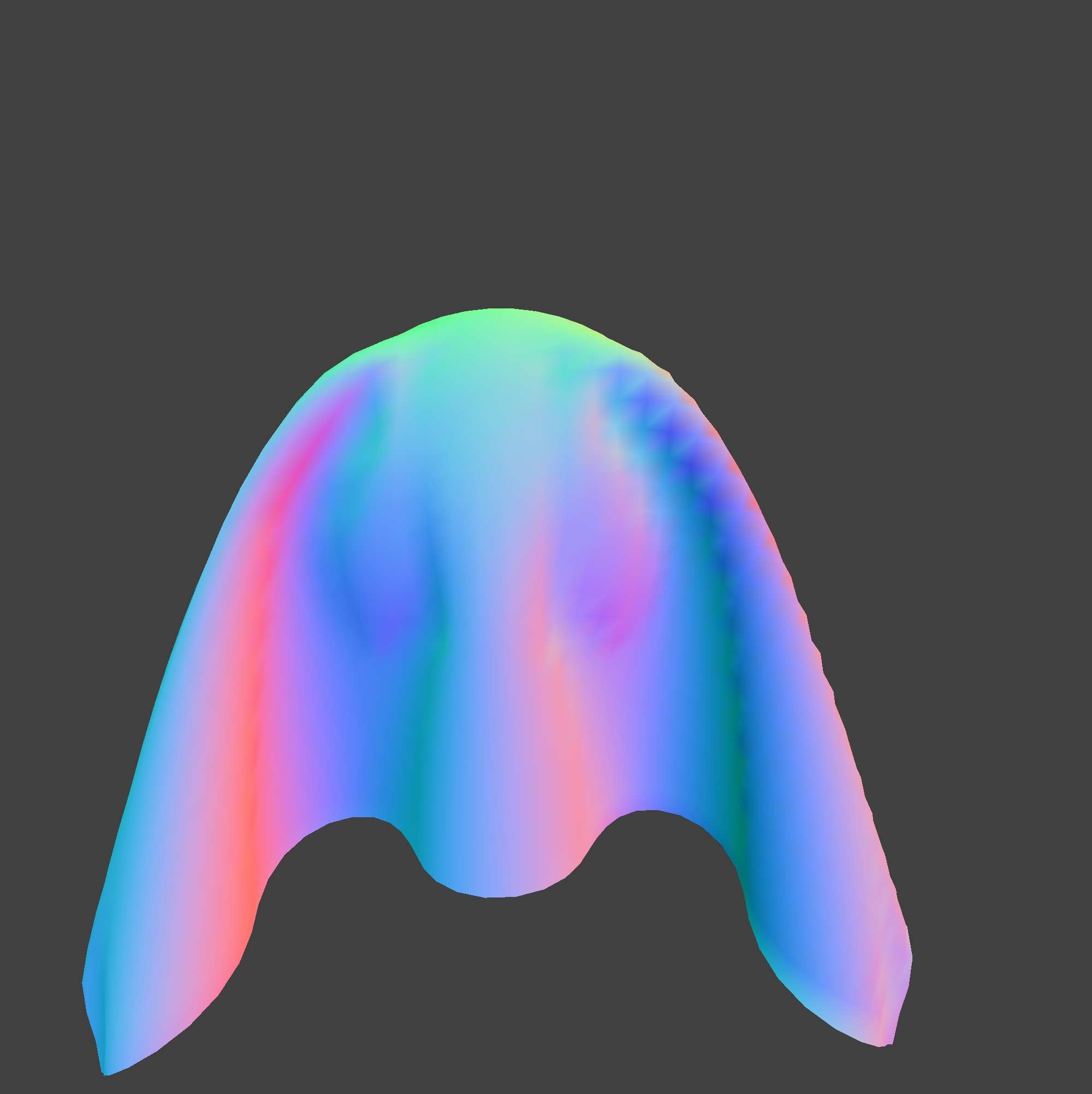
The first row shows the final rest state of the cloth on the sphere, along with the simulation video. The second row shows the cloth resting on the sphere with ks=500 and ks=50000. We can see that with a lower spring constant, the cloth is more loose and falls more smoothly on the sphere, while with a higher spring constant, the cloth is stiffer and has more resistance to deformation. This means the cloth is picking up off the sphere more, and the bends are wider.
Plane Collision
In my implementation of the plane collision detection algorithm, I calculate the vector from the plane point to the last and current positions of the point mass. I check if the point mass has crossed the plane by checking if the vectors have different signs. If the point mass has crossed the plane, I calculate the projection of the current position onto the plane and find the tangent point. I then calculate the correction vector needed to be applied to the point mass’s last position in order to reach a point slightly above the tangent point, on the same side of the plane that the point mass was before crossing over. Finally, I apply the correction with a small offset and update the position of the point mass.
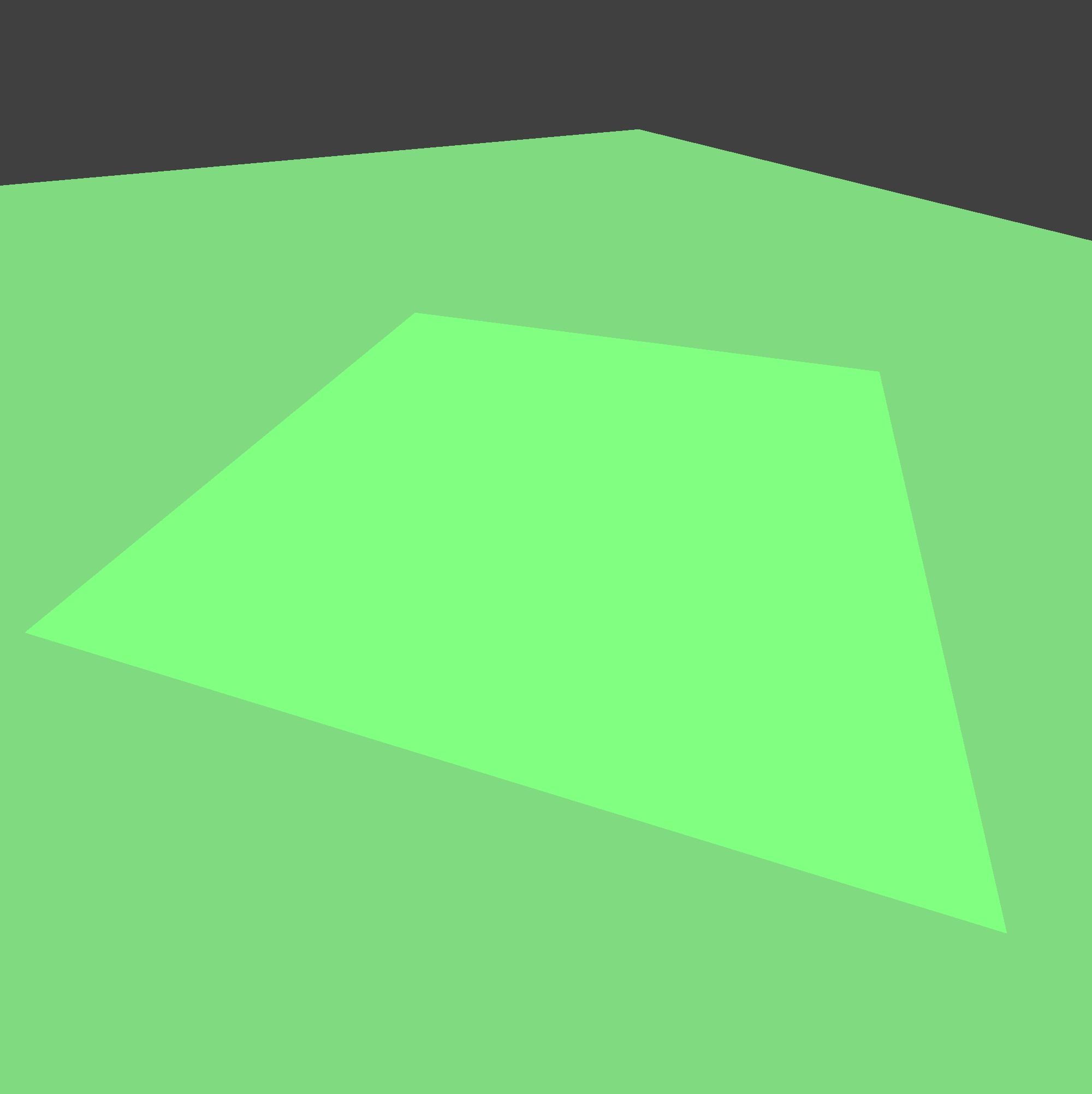
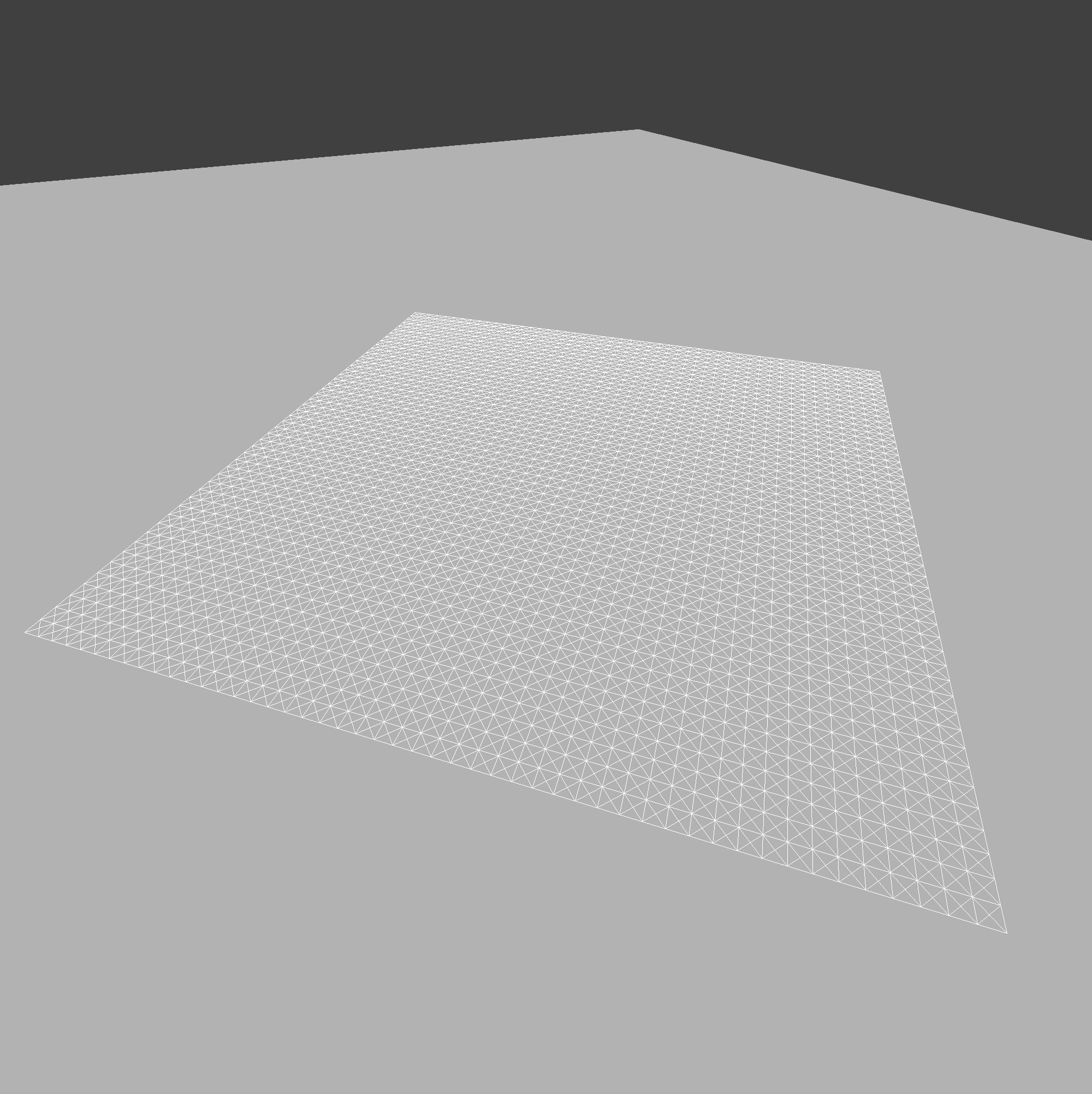
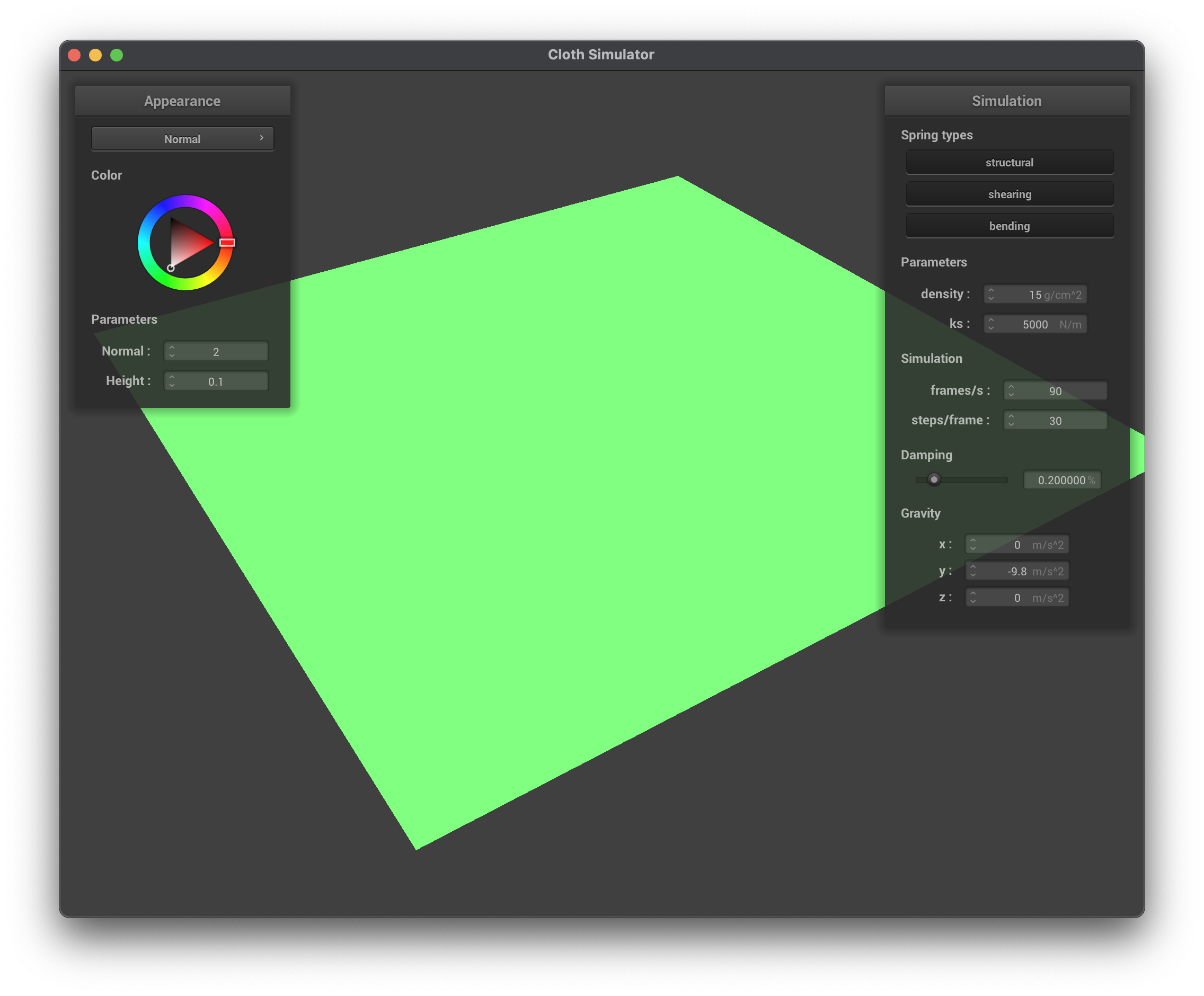
The first image shows the cloth laying on the plane with normal shading, while the second image shows the wireframe of the cloth on the plane.
Handling Self-Collisions
Next, we want to prevent the cloth from passing through itself. To do this, we need to check for self-collisions between point masses and apply a correction to their positions if they are colliding.
To start, we need to develop a hashing function that maps the point masses to a grid of cells. This will allow us to efficiently check for collisions between point masses that are close to each other.
In my implementation, I used a hash function that takes the position of the point mass and maps it to a unique float identifier that represents membership in some 3D box volume. The box dimensions are calculated based on the width and height of the cloth and the number of point masses in each dimension. The hash function partitions space into 3D boxes, with dimensions w, h, and t, where w is 3 times the width divided by the number of width points, h is 3 times the height divided by the number of height points, and t is the maximum of w and h.
The hash function then calculates which box the position by taking the floor of the position divided by the box dimensions. By combining the indices of the box with a large number multiplied by the max number of dimensional points, we can achieve a x-y-z hash value, akin to row major vectors, that is unique to the box. This allows us to efficiently check for collisions between point masses that are in the same box.
Next, we need to check for self-collisions between point masses. For each point mass, we check if it is colliding with any other point masses in the same box. If it is, we calculate the distance between the two point masses and check if it is less than twice the thickness of the cloth. If it is, we apply a correction to the position of the point mass to push it away to the desired distance. Then we average the correction vector with the other colliding point masses and scale it by the number of simulation steps to prevent the cloth from passing through itself.
The following images show the cloth at different stages of self-collision, including an early self-collision, ongoing folding, and final resting state.
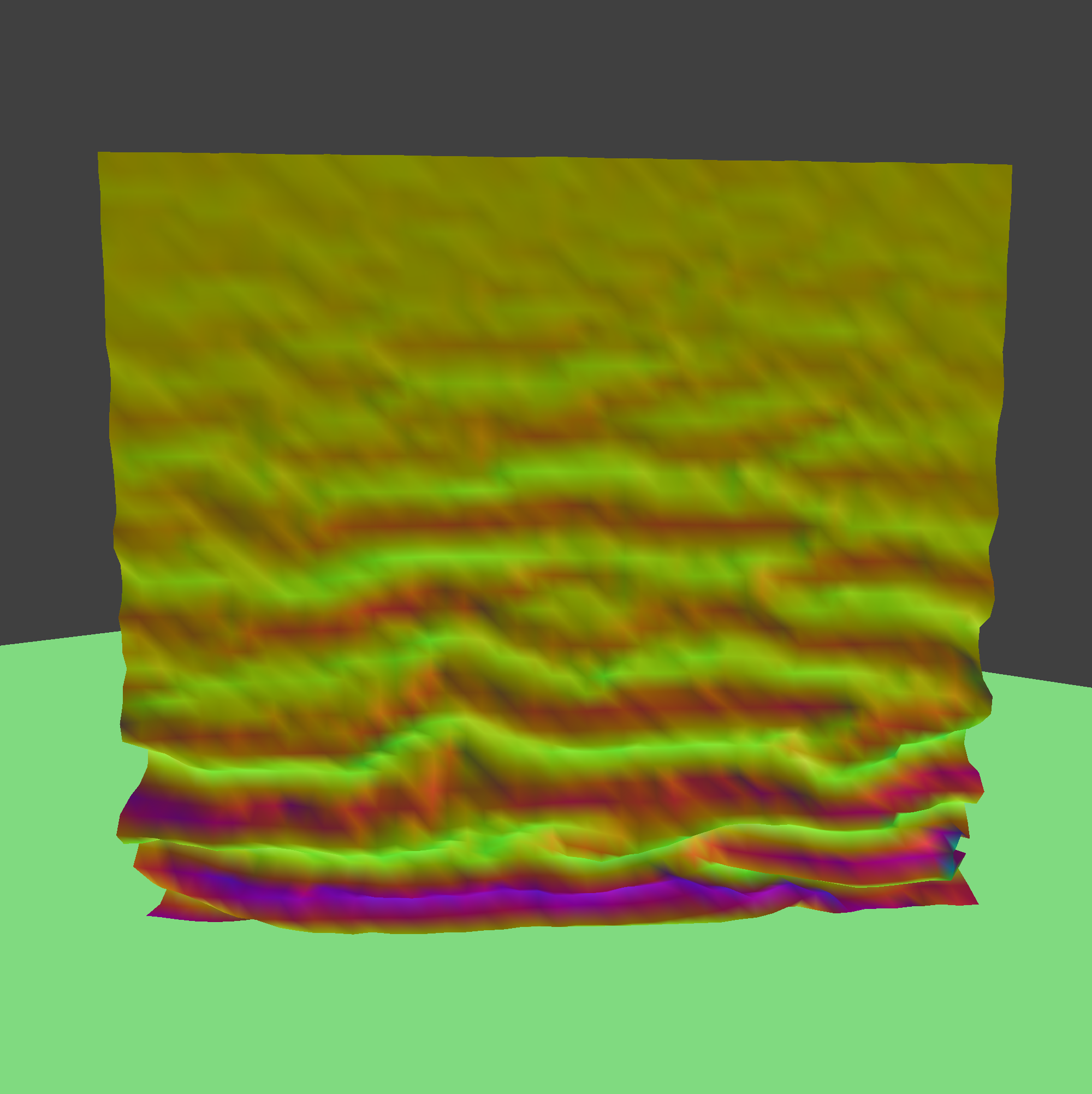
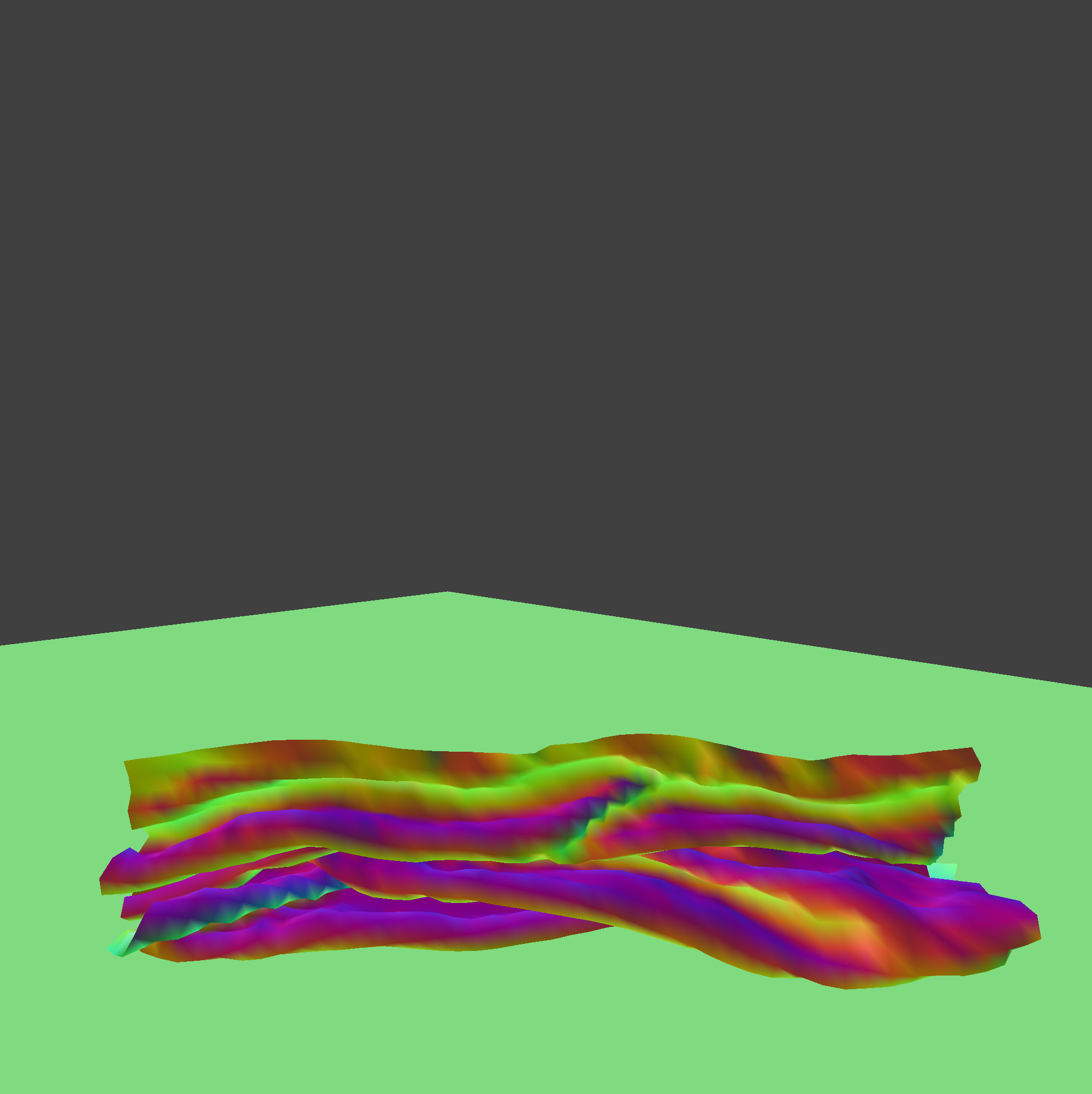
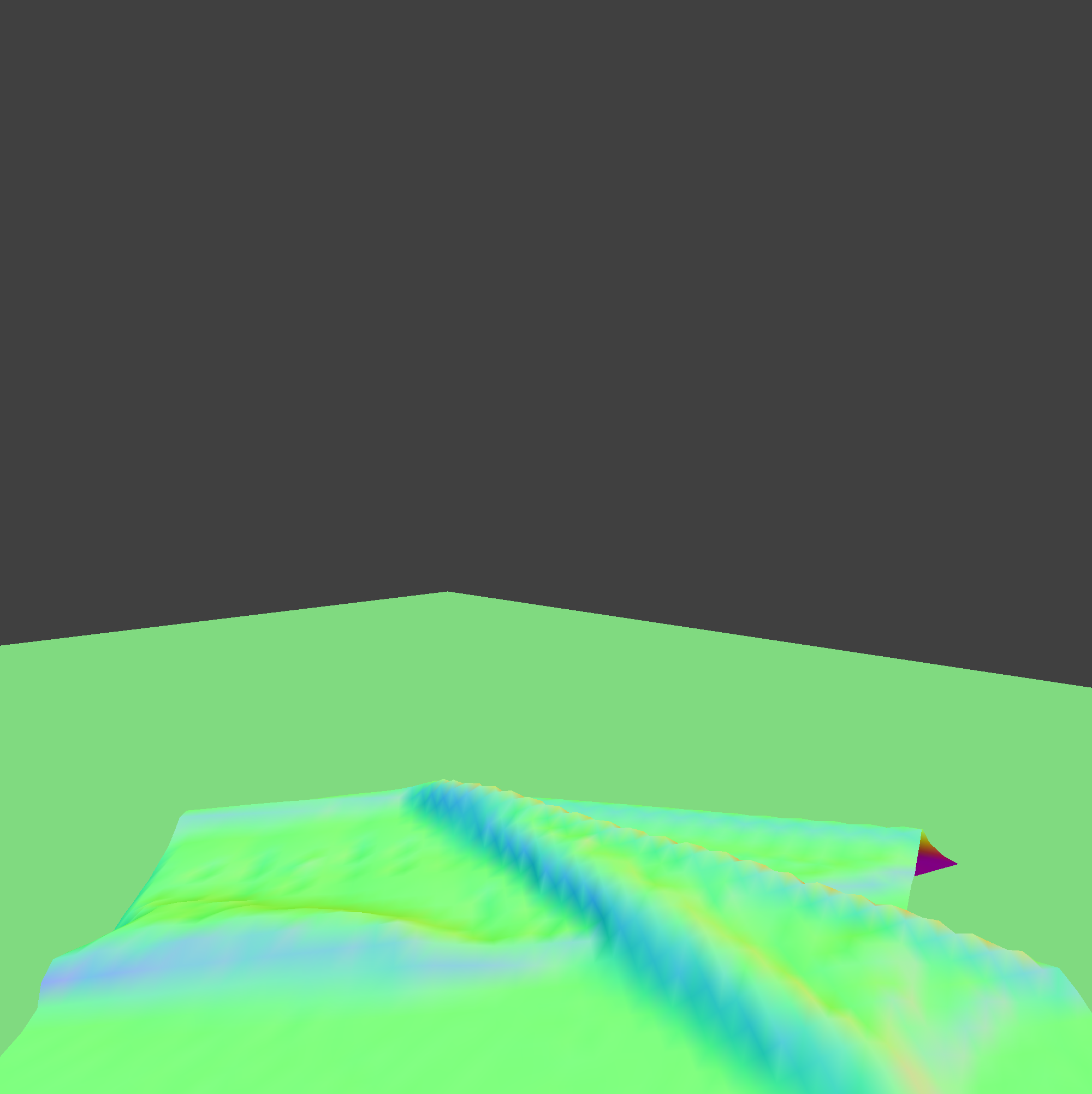
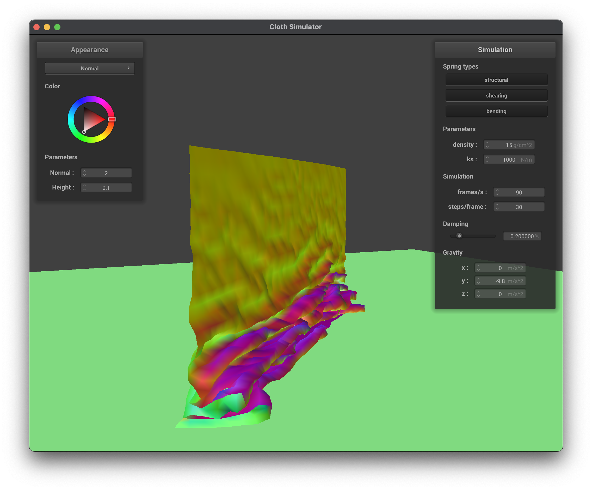
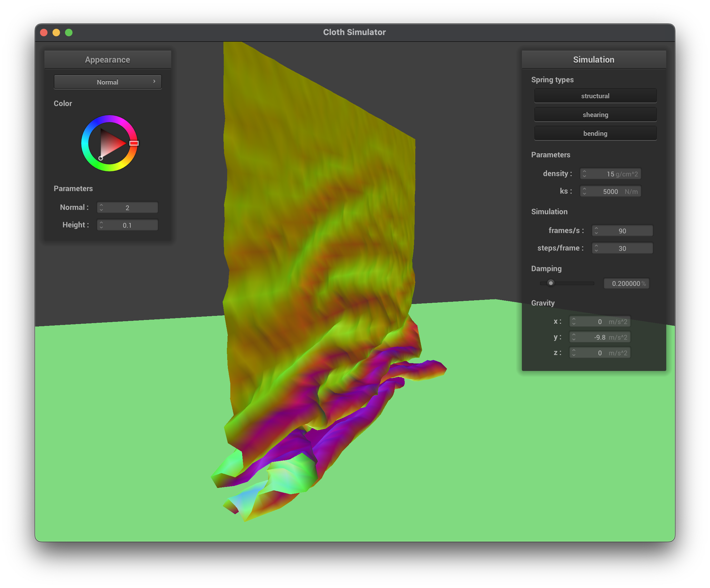
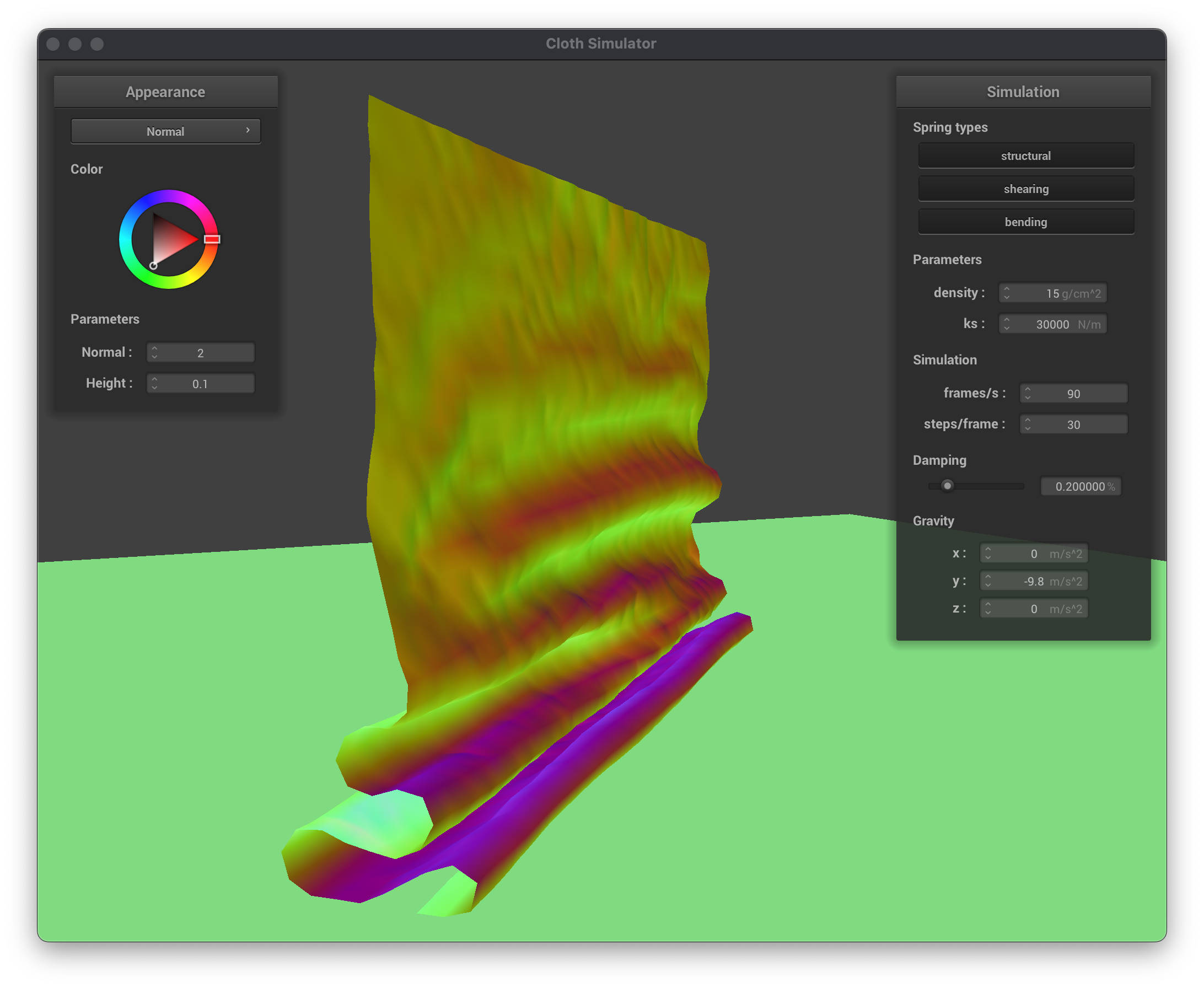
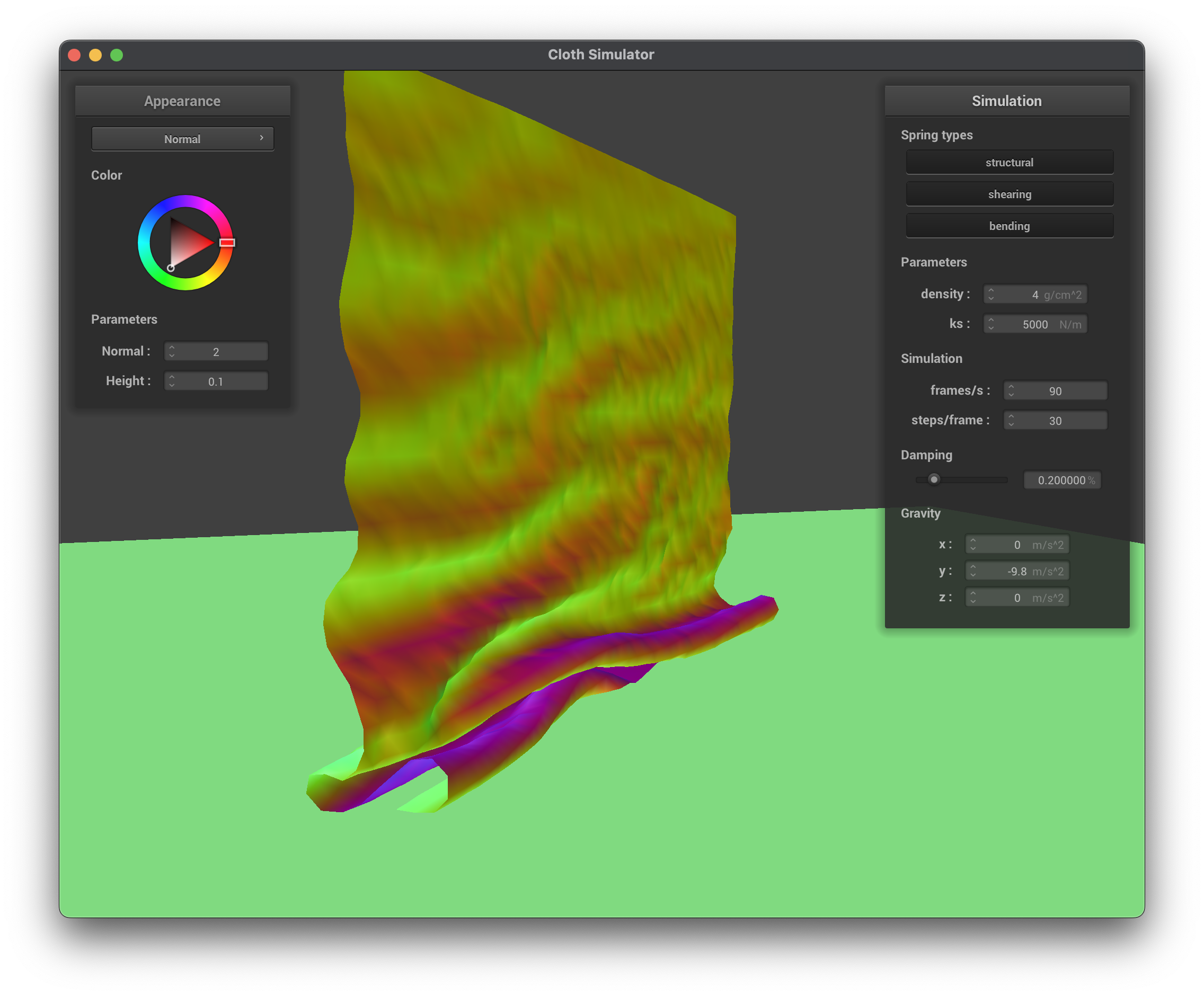
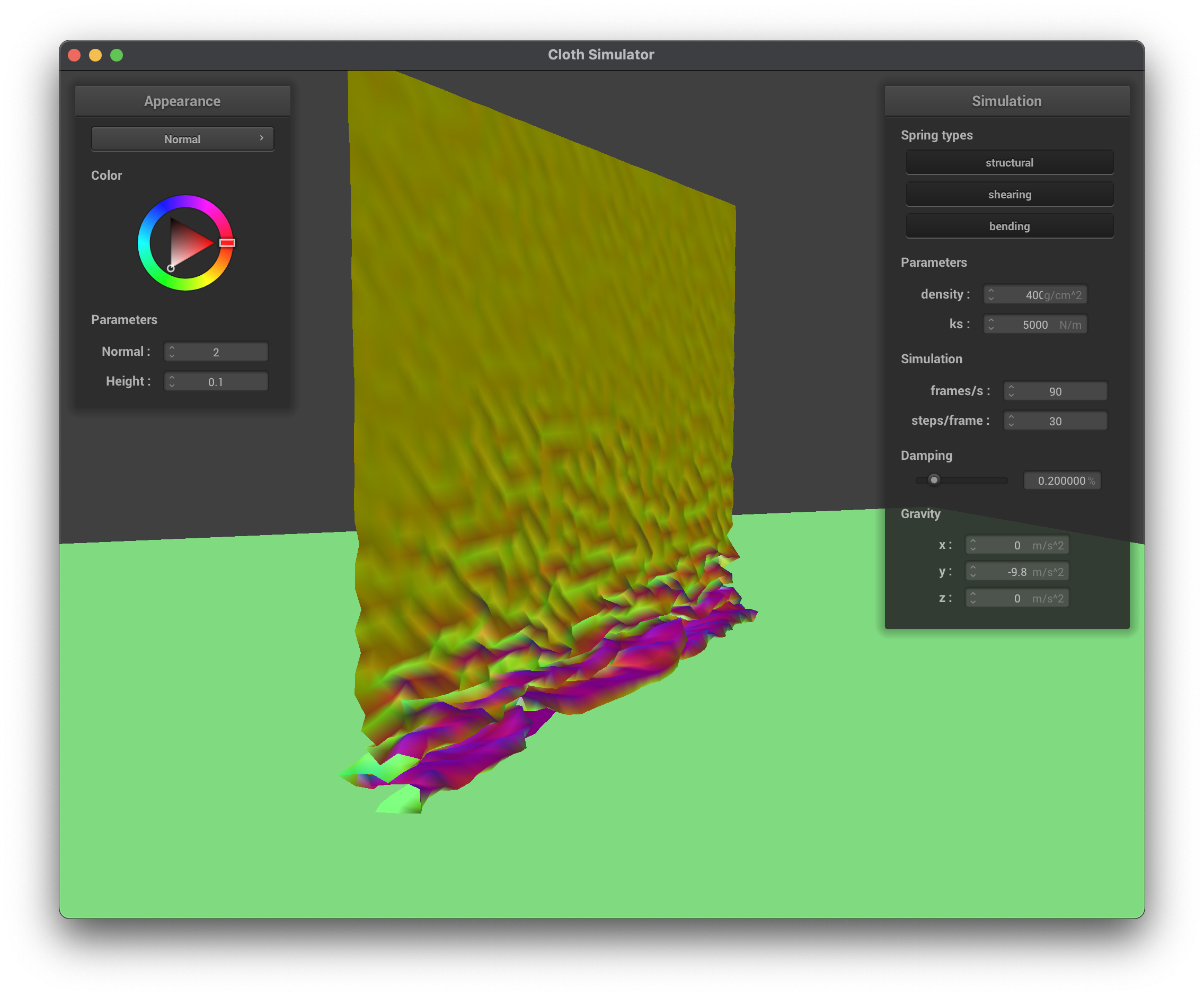
The middle row shows the cloth mid compresion with different spring constants, ks=1000, ks=5000, and ks=30000. We can see that with a lower spring constant, the cloth is more loose and the fold patter on the ground is quite loose, while as the constant increases, the folds become stronger and support more of the weight above. The video shows the simulation video of the cloth self-colliding and folding on itself.
The last row shows the cloth with different densities, density=4 and density=400. We can see that with a lower density, the cloth has the same properties as a stronger spring constant, where the folds are more pronounced and the cloth is not collapsing on itself as much. With a higher density, the cloth is heavier and falls faster, resulting in more pronounced folds, wrinkles, and self-collisions. Surprisingly, I noted how in a high density the top of the cloth is more resilient to the folding while falling, while in a less dense fabric the folding begins very early on in the top section.
Shaders
A shader program is a small program executed on the GPU to control how vertices and fragments (pixels) are processed and rendered on screen. A shader program is typically composed of at least a vertex shader and a fragment shader:
- Vertex Shader: It processes each vertex, applying transformations (such as model, view, projection), performing per-vertex operations, and passing per-vertex data (like normals, texture coordinates) to subsequent stages.
- Fragment Shader: It computes the final pixel color by taking the interpolated data from the vertex shader, performing lighting calculations, material effects, and texture lookups.
Together, these shaders work to create a variety of lighting and material effects. The vertex shader defines the shape and position of 3D geometry, while the fragment shader colors that geometry based on lighting models, textures, and other visual effects.
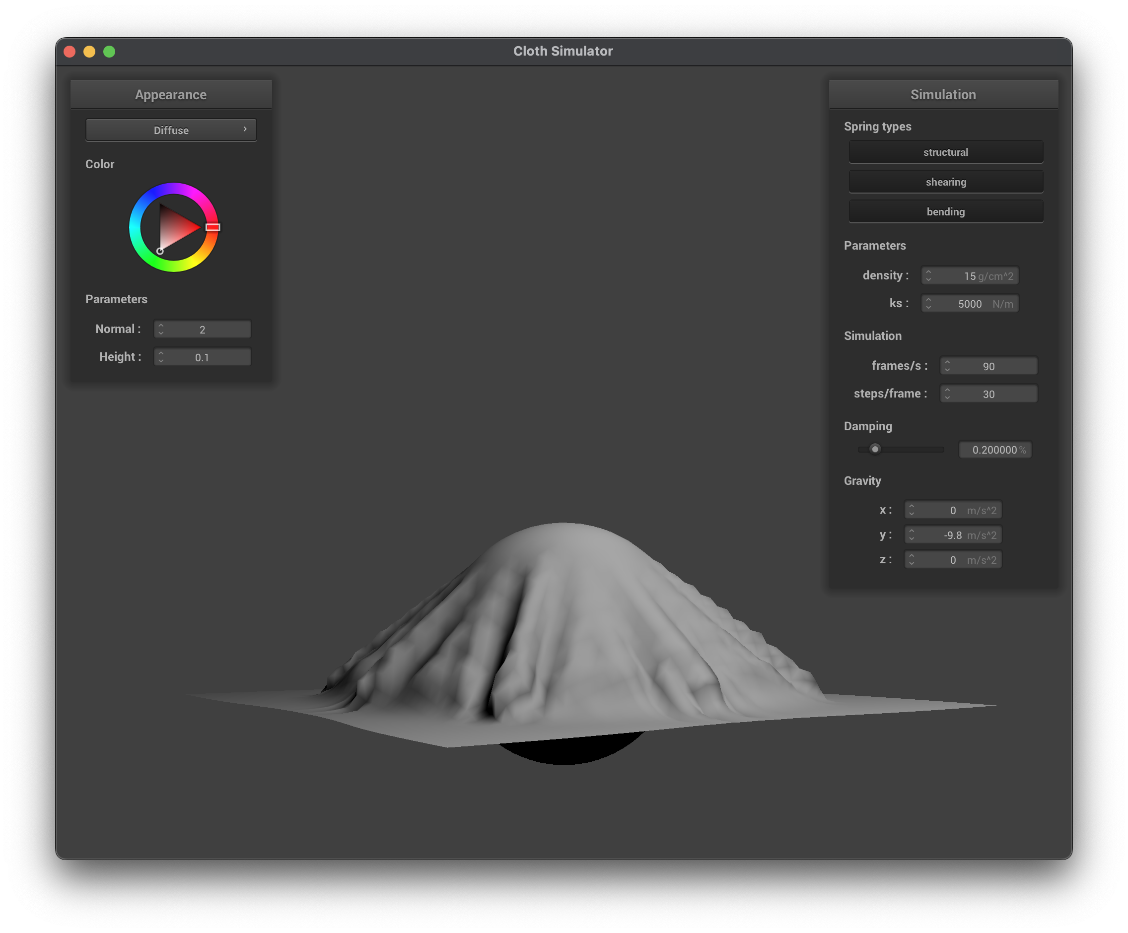
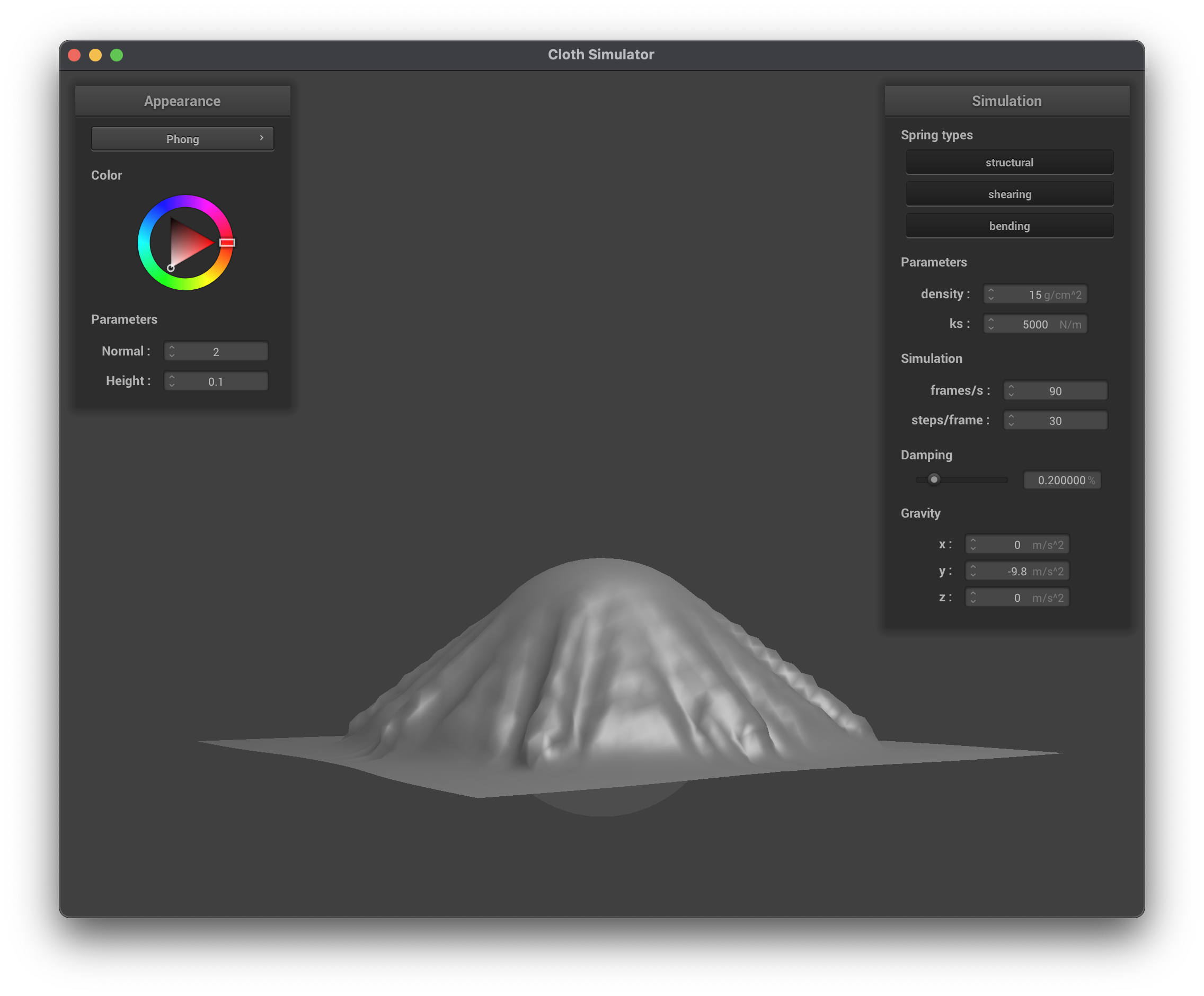
Here are some examples of the shaders I implemented:
Diffuse Lighting Shader
The diffuse mapping shader uses the Lambertian reflectance model to simulate the diffuse reflection of light on a surface. The shader computes the diffuse color based on the angle between the surface normal and the light direction, which is determined by the dot product of the two vectors. The diffuse color is then scaled by the light intensity and the color of the light source.
Blinn–Phong Shader
The Blinn–Phong shading model has three main components:
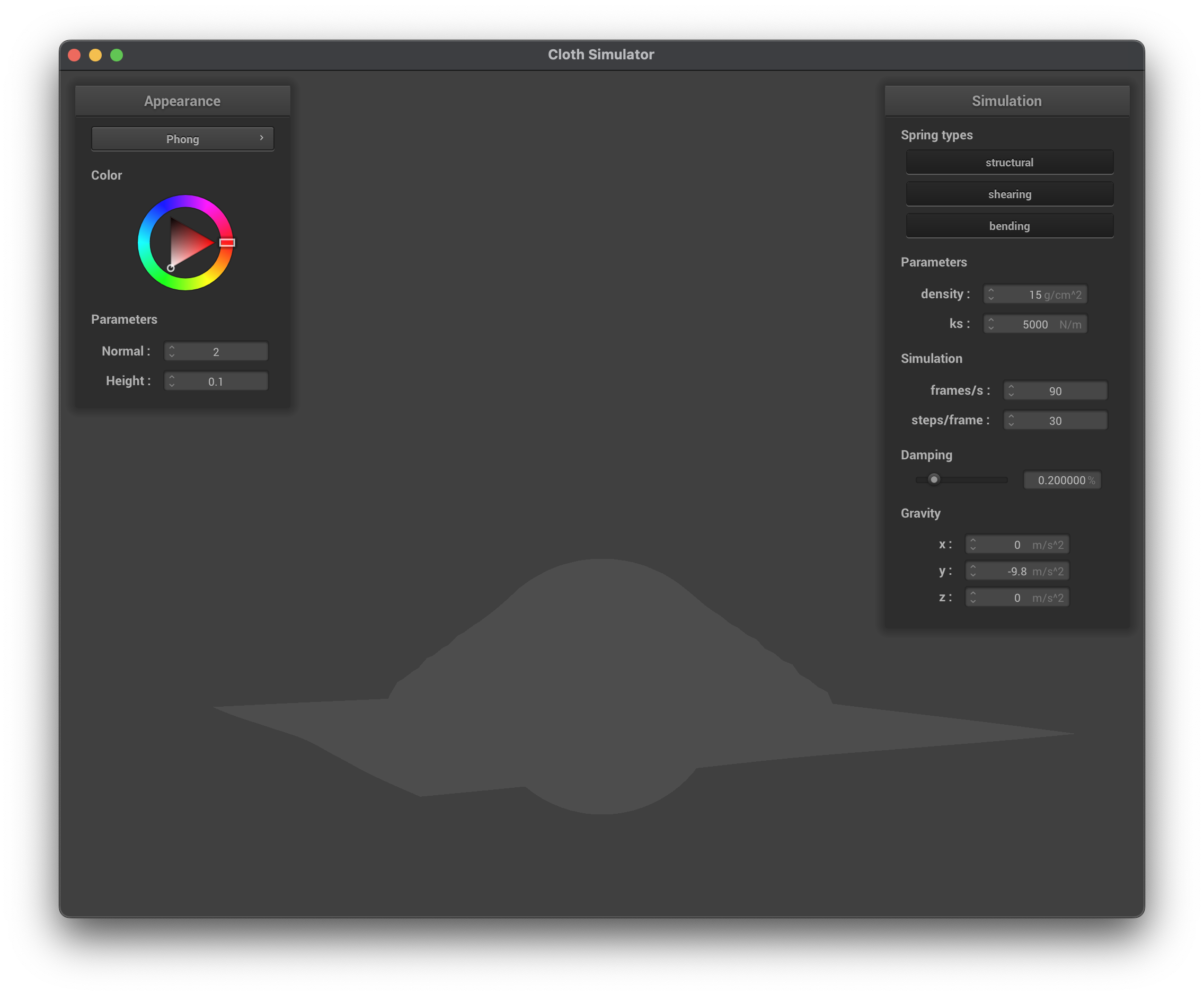
- Ambient: A constant term that ensures objects are visible even with no direct lighting.
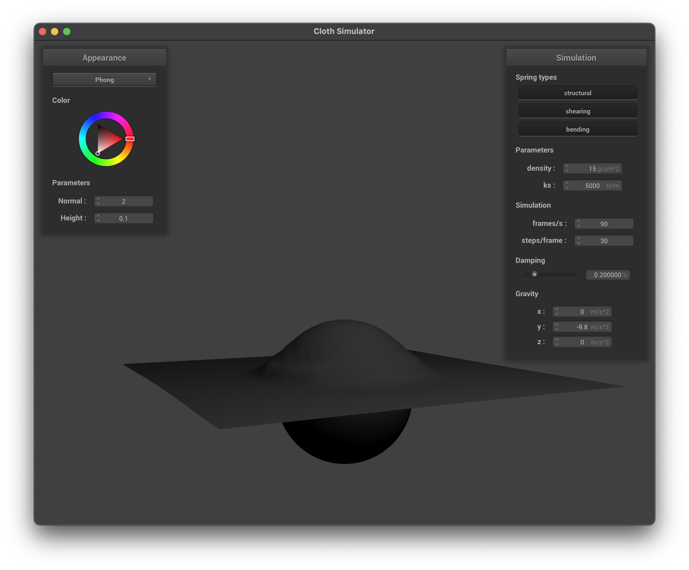
- Diffuse: Simulates the matte, scattered reflection of light from a surface. It depends on the angle between the surface normal and the light direction.
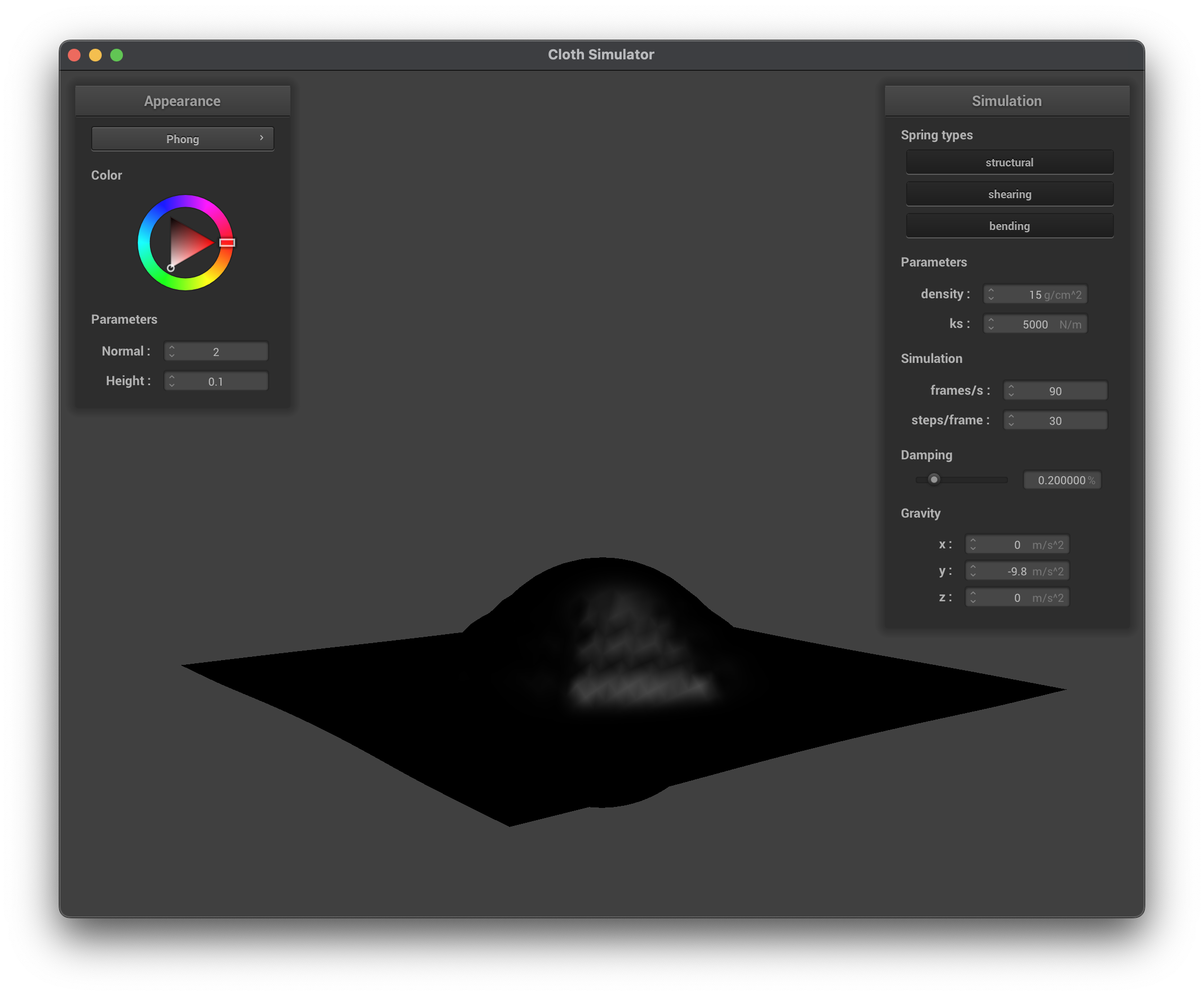
- Specular: Models the shiny highlights on reflective surfaces. In Blinn–Phong, this is computed using the half vector (which is the average between the light direction and view direction).
We can visualize the contributions of each component in the Blinn–Phong model. The following images show the results of rendering with only the ambient, diffuse, specular components, and finally the full Blinn–Phong model:

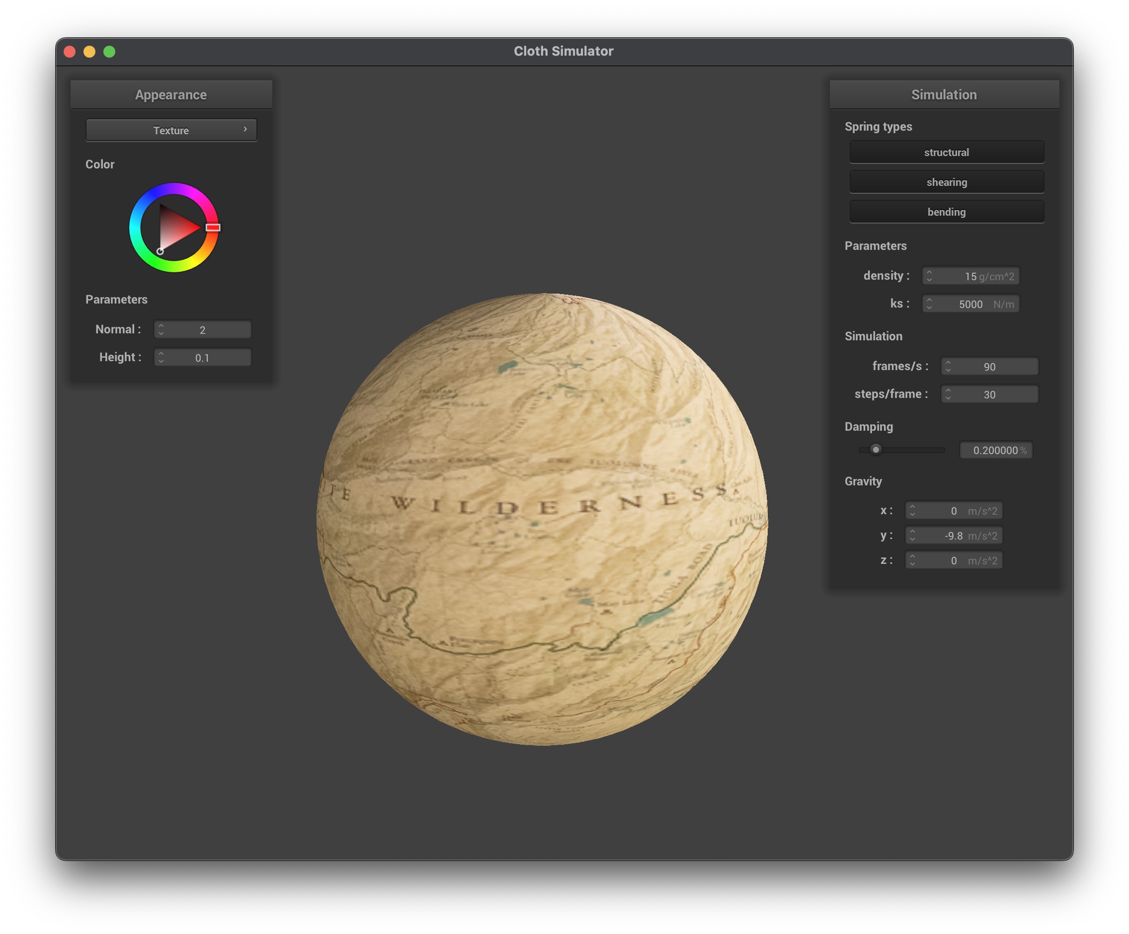
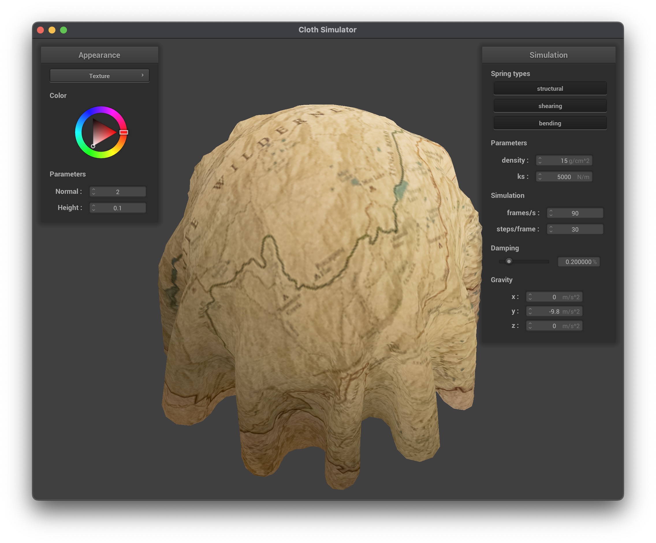
Texture Mapping Shader
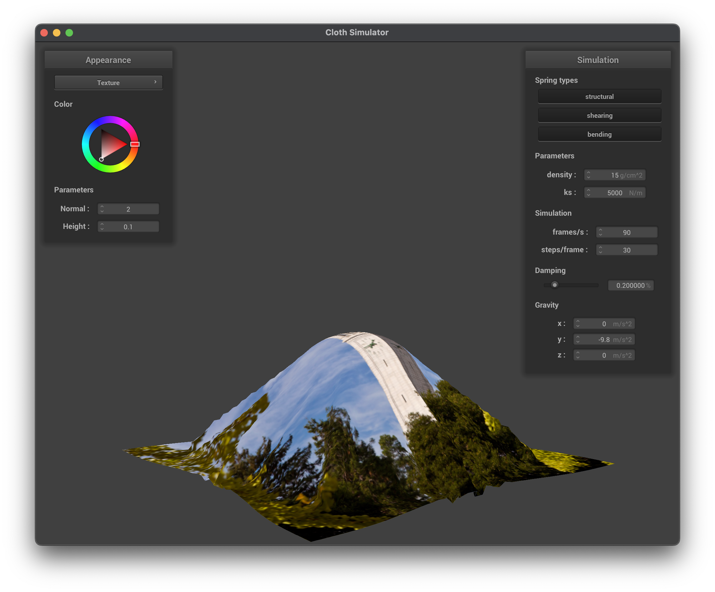
Texture mapping is a technique used to apply a 2D image (texture) onto a 3D surface. The shader can sample from a texture using the built-in function texture(sampler2D tex, vec2 uv), which retrieves the color from the texture at the specified UV coordinates. Luckily, the texture coordinates are already provided in the vertex shader, so we can directly use them in the fragment shader to sample the texture.
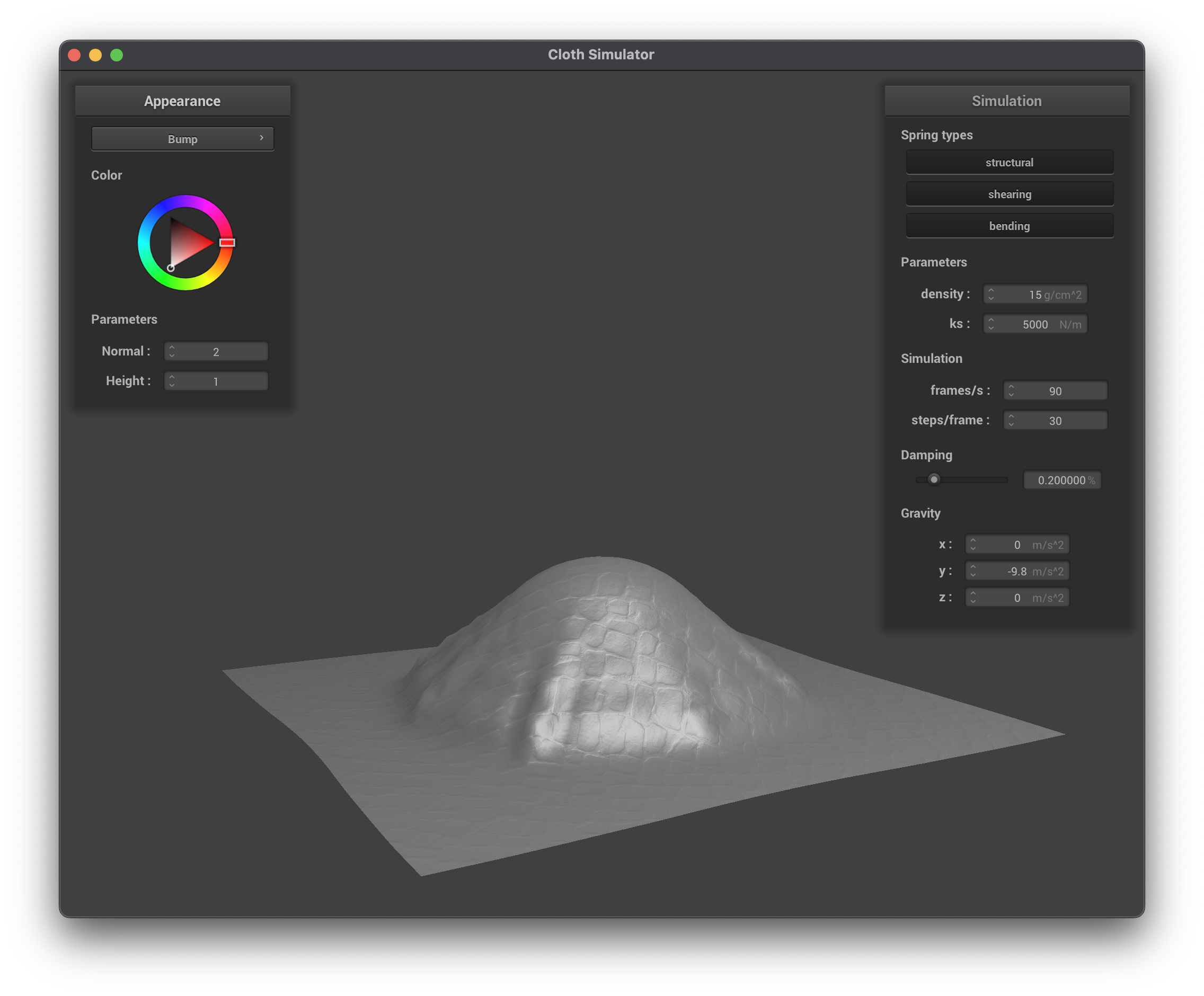
Bump Mapping and Displacement Mapping Shader
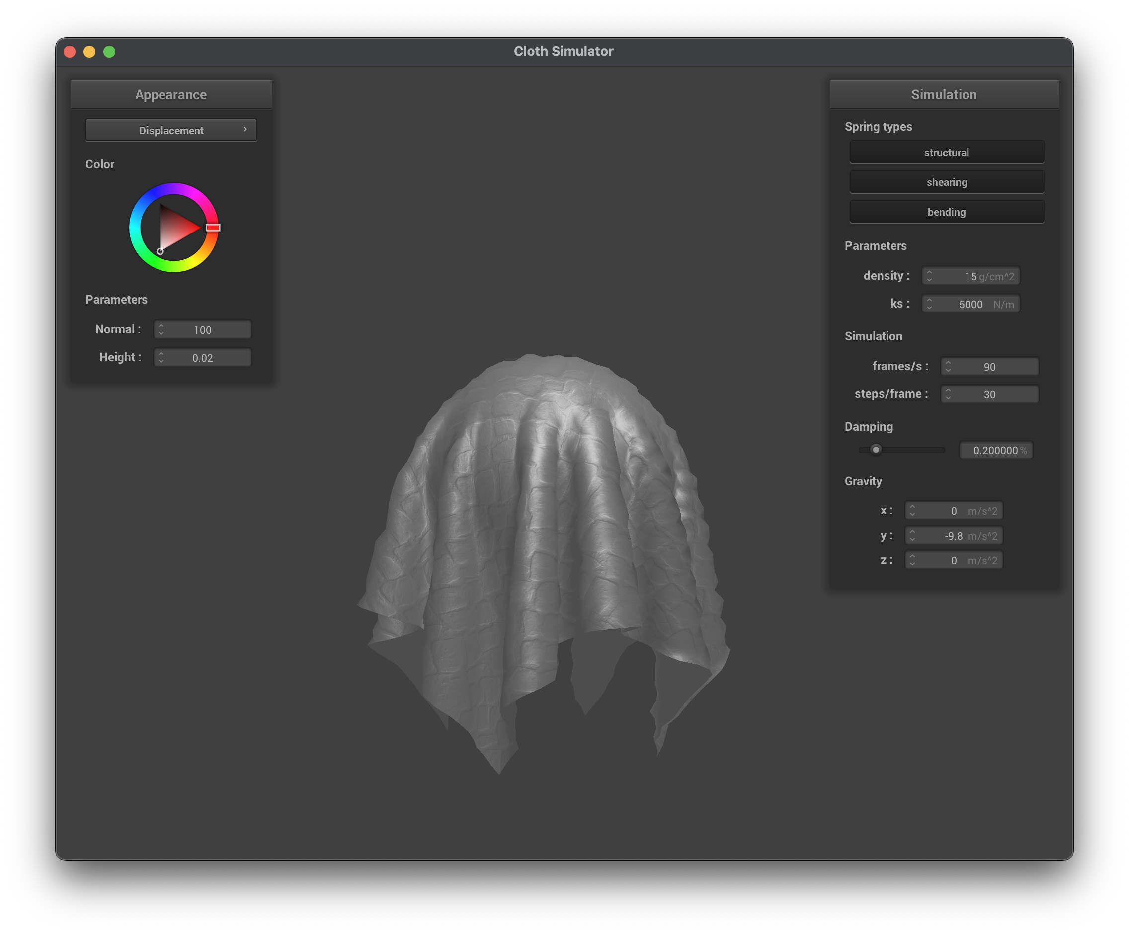
Bump mapping is used to perturb the normals across the surface without changing the actual geometric position. This gives the illusion of small-scale details such as wrinkles or bumps. Displacement mapping does the same, but also physically moves the vertices along the normal based on the height map, creating actual geometric detail:
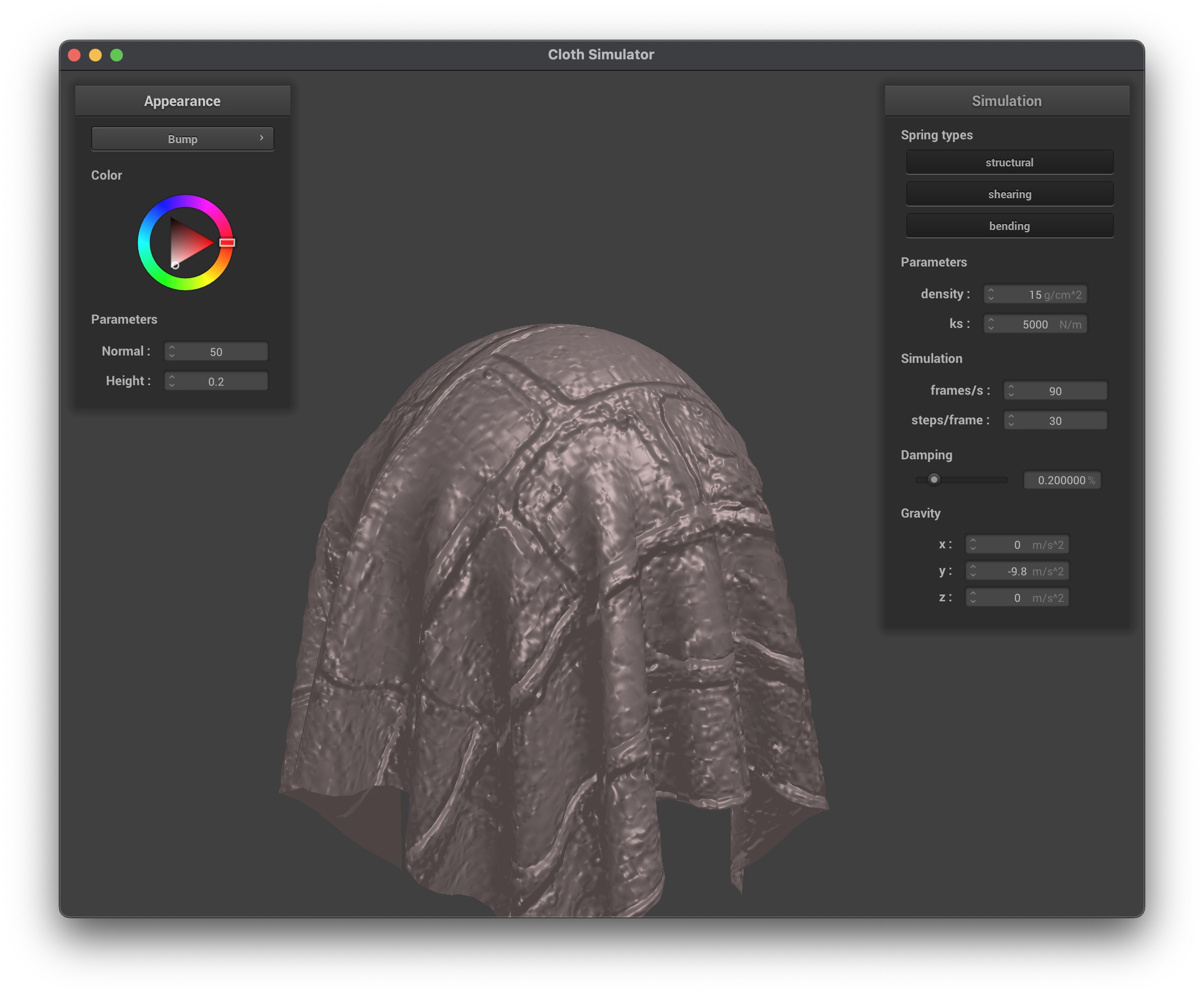
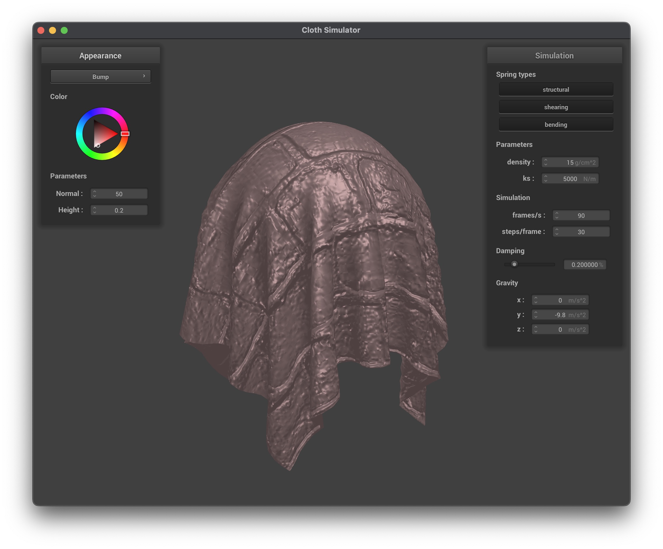
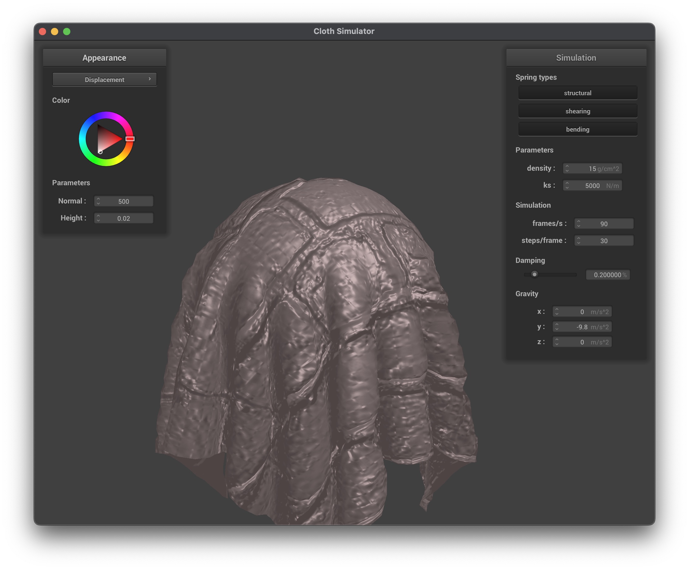
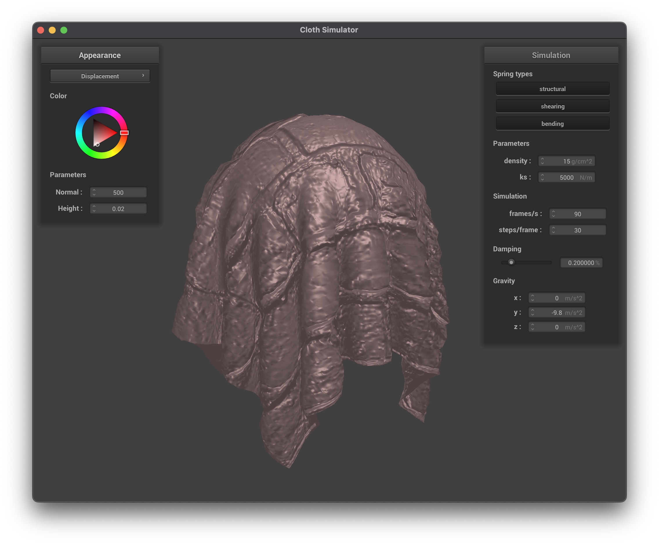
In the higher resolution spheres, we can see how the bump mapping illusion does not hold up as well, as the underlying sphere is much smoother than the lower resolution sphere. However, displacement mapping is not affected by the resolution of the sphere, as it actually modifies the vertex positions based on the height map so the details are preserved regardless of the resolution.
- Bump Mapping:
- Pros: Faster, since only normals are perturbed; no extra geometry is added.
- Cons: Only the illusion of detail is provided; silhouettes remain unchanged.
- Displacement Mapping:
- Pros: Provides true geometric detail with altered silhouettes.
- Cons: More computationally expensive as vertex positions are modified.
Mirror Shader
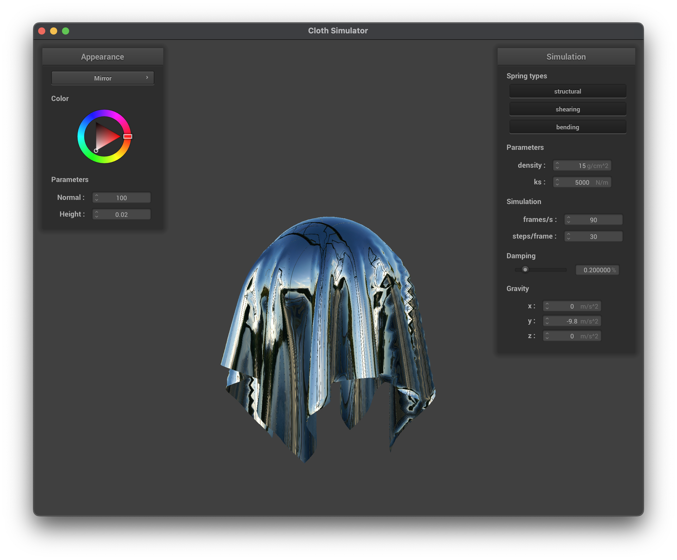
The mirror shader uses an environment map to simulate perfect reflections by reflecting the eye-ray off the surface. Below are the results:
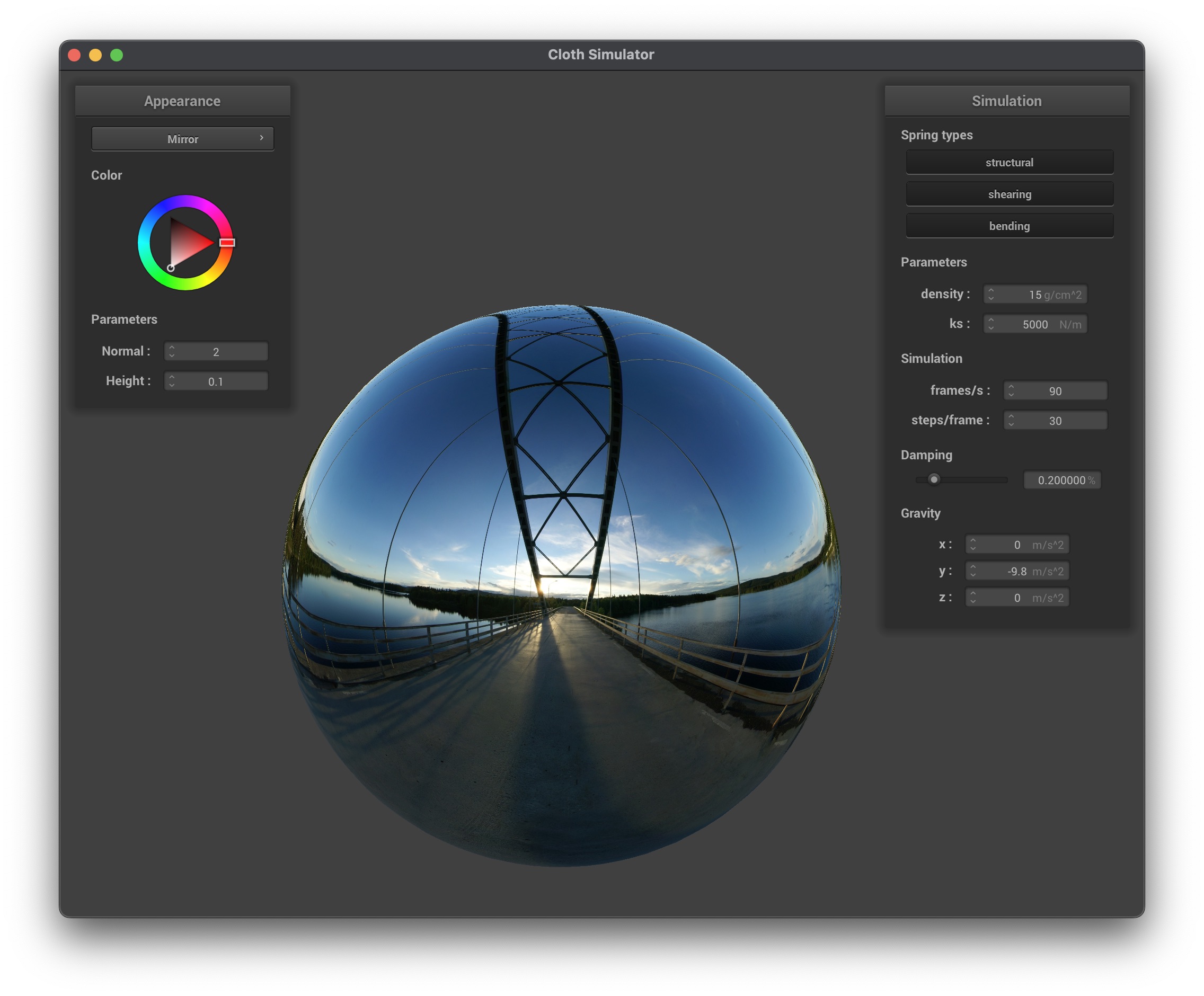
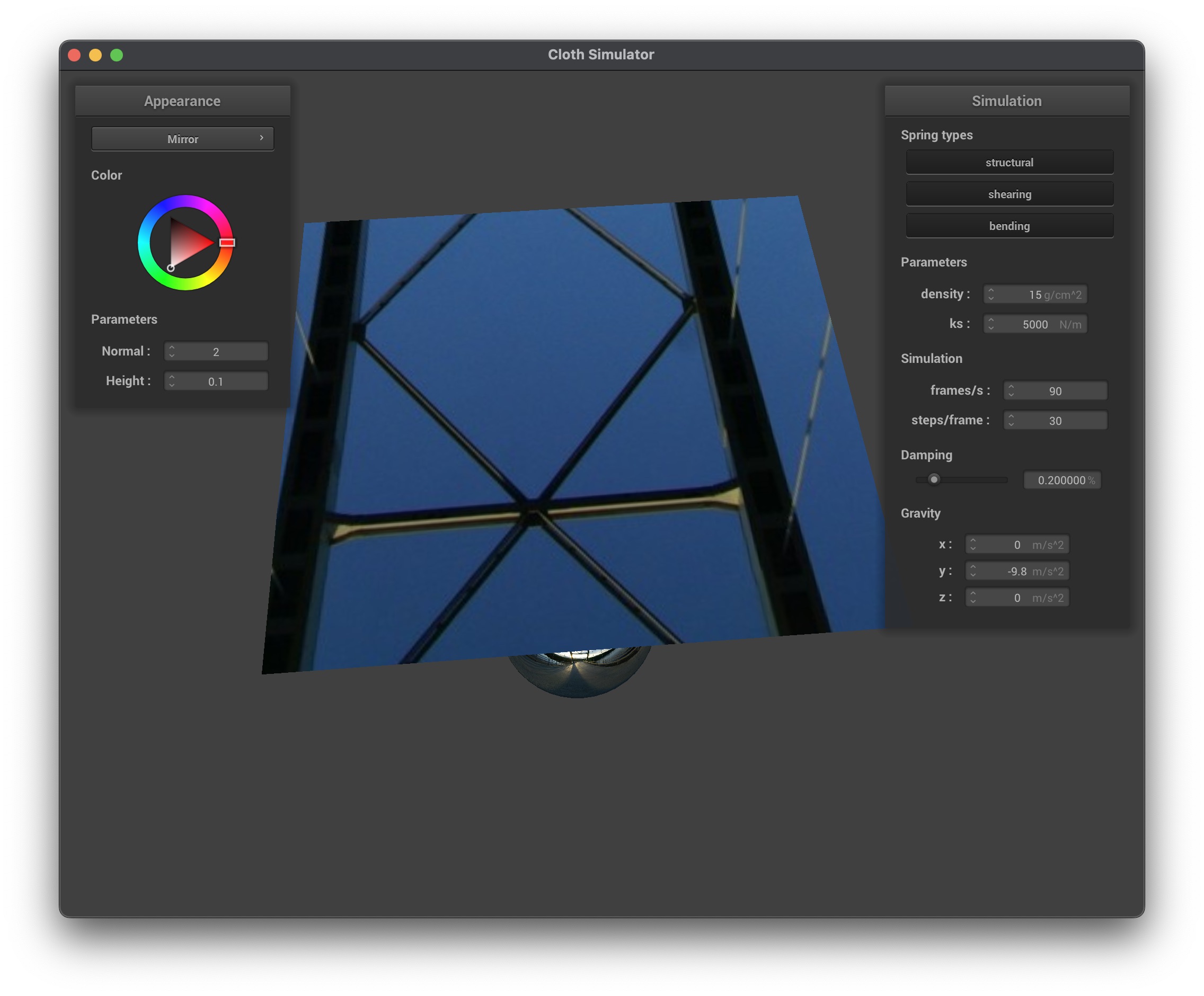
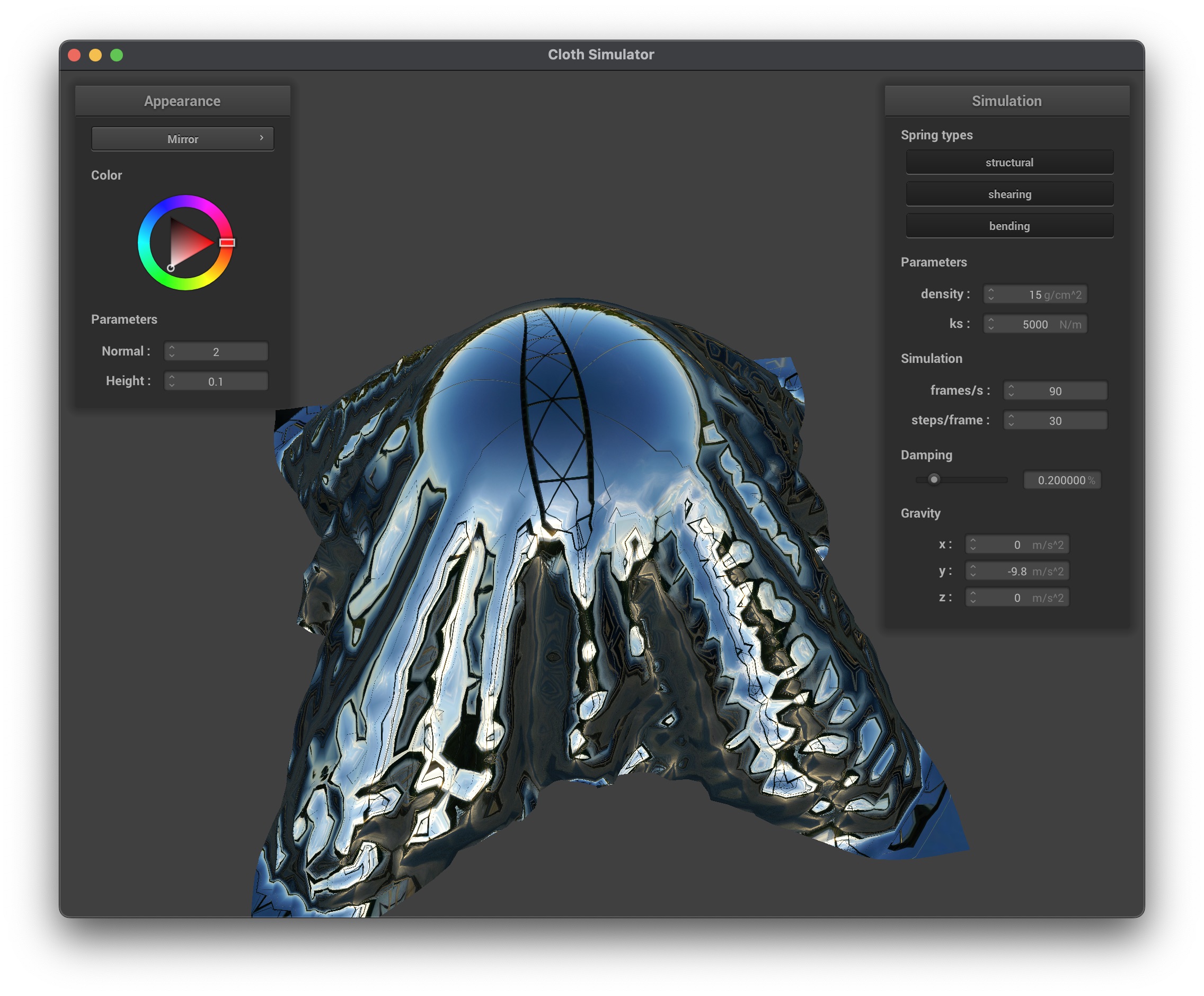
You can see how the mirror shader creates a perfect reflection of the environment on the sphere and the cloth. The flat cloth shows a clear reflection of the environment, while the falling cloth shows a distorted reflection due to its dynamic shape.
Custom Shader
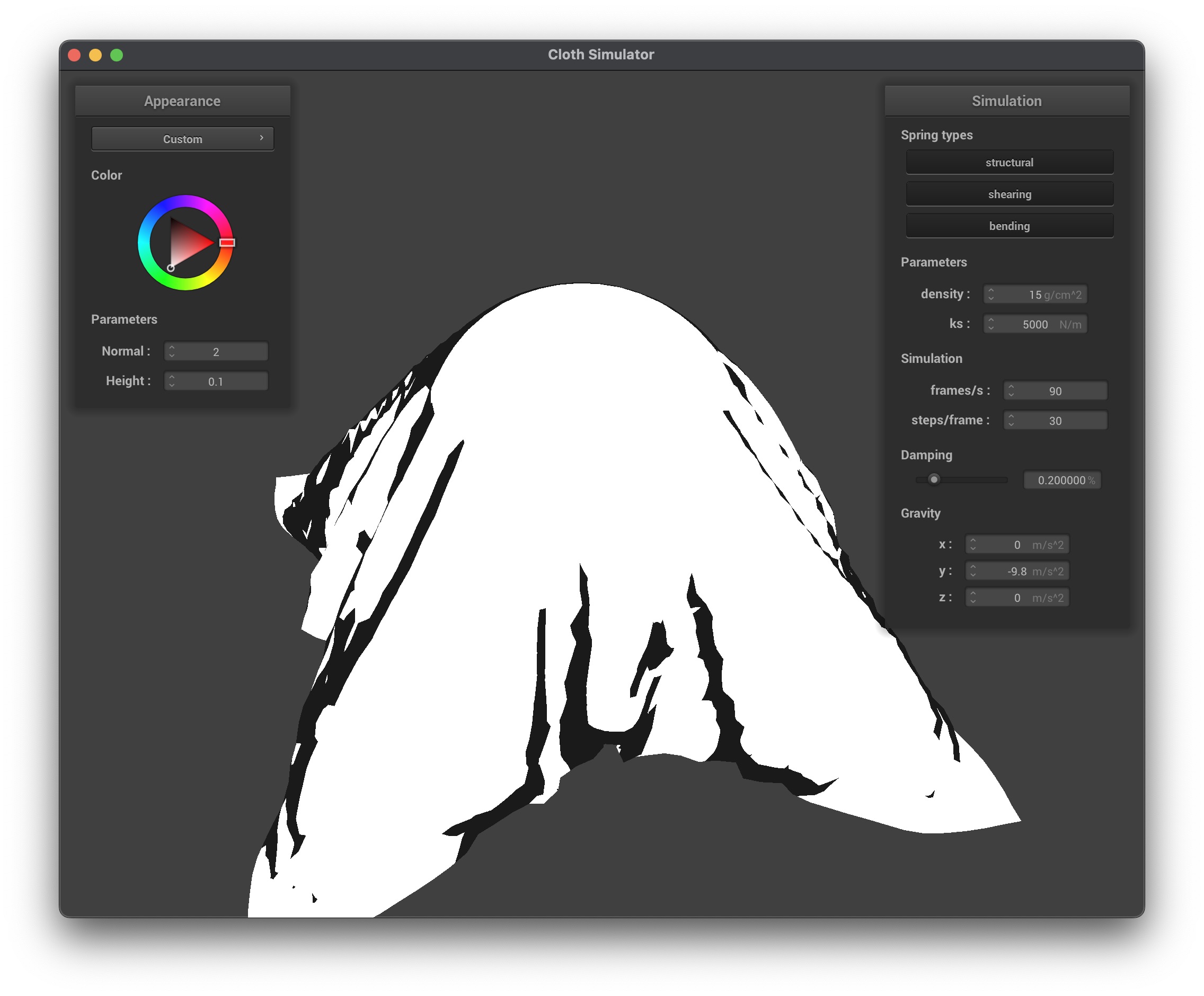
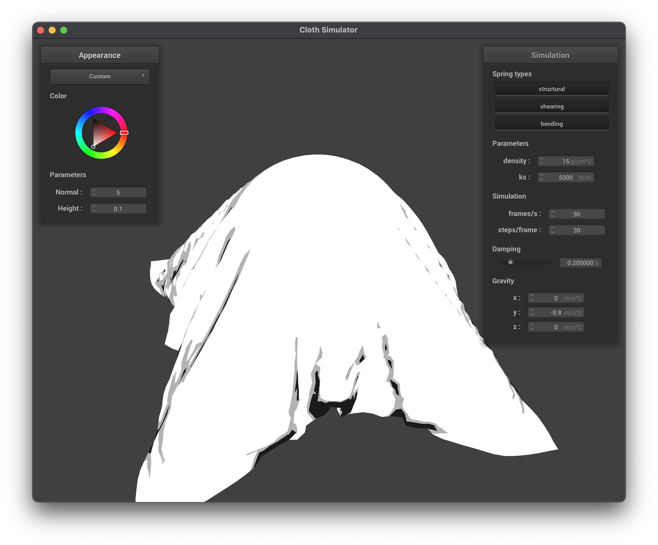
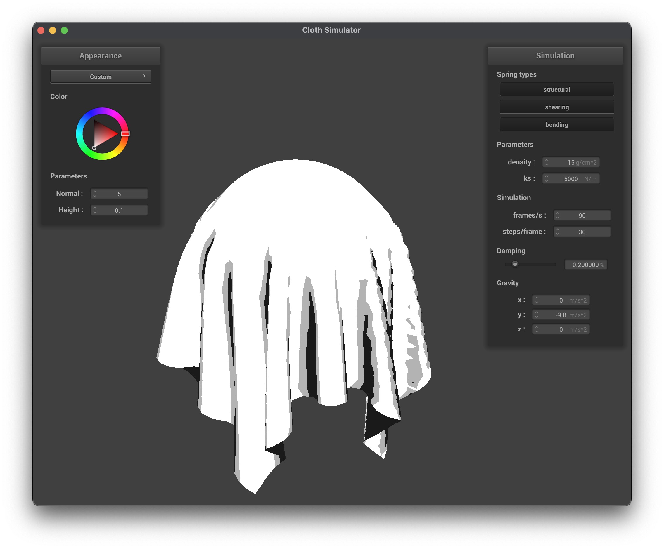
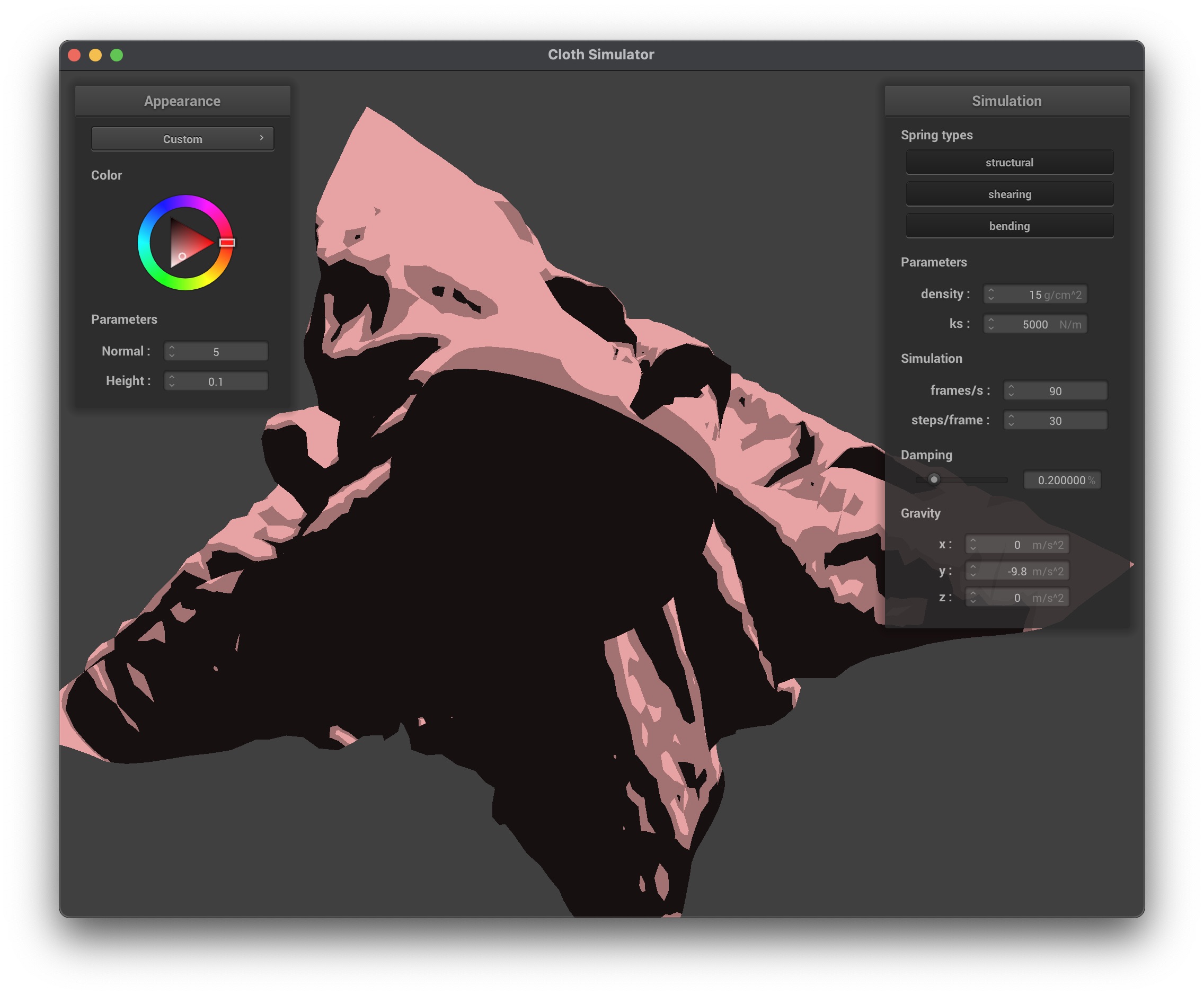
In my custom shader, I created a Blinn–Phong cell shading effect. The key modifications I made were:
- Quantization: I quantized both the diffuse and specular components using the
u_normal_scalingas a method to change the desired number of colors, which results in discrete lighting steps. This gives the appearance of cartoon-like shading. - Combination: I combined ambient, diffuse, and specular terms to form the final shaded output and then modulated that result with the base material color (
u_color).
This approach allowed for a stylized rendering where lighting appears broken into distinct bands rather than smooth gradients, which is characteristic of cel shading.
